R for Deep Learning (I): Build Fully Connected Neural Network from Scratch

Backgrounds

Deep Neural Network (DNN) has made a great progress in recent years in image recognition, natural language processing and automatic driving fields, such as Picture.1 shown from 2012 to 2015 DNN improved IMAGNET’s accuracy from ~80% to ~95%, which really beats traditional computer vision (CV) methods.

Picture.1 - From NVIDIA CEO Jensen’s talk in CES16

In this post, we will focus on fully connected neural networks which are commonly called DNN in data science. The biggest advantage of DNN is to extract and learn features automatically by deep layers architecture, especially for these complex and high-dimensional data that feature engineers can’t capture easily, examples in Kaggle. Therefore, DNN is also very attractive to data scientists and there are lots of successful cases as well in classification, time series, and recommendation system, such as Nick’s post and credit scoring by DNN. In CRAN and R’s community, there are several popular and mature DNN packages including nnet, nerualnet, H2O, DARCH, deepnet and mxnet, and I strong recommend H2O DNN algorithm and R interface. 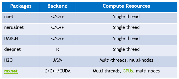So, why we need to build DNN from scratch at all? - Understand how neural network works Using existing DNN package, you only need one line R code for your DNN model in most of the time and there is an example by neuralnet. For the inexperienced user, however, the processing and results may be difficult to understand. Therefore, it will be a valuable practice to implement your own network in order to understand more details from mechanism and computation views. - Build specified network with your new ideas DNN is one of rapidly developing area. Lots of novel works and research results are published in the top journals and Internet every week, and the users also have their specified neural network configuration to meet their problems such as different activation functions, loss functions, regularization, and connected graph. On the other hand, the existing packages are definitely behind the latest researches, and almost all existing packages are written in C/C++, Java so it’s not flexible to apply latest changes and your ideas into the packages. - Debug and visualize network and data As we mentioned, the existing DNN package is highly assembled and written by low-level languages so that it’s a nightmare to debug the network layer by layer or node by node. Even it’s not easy to visualize the results in each layer, monitor the data or weights changes during training, and show the discovered patterns in the network.

Fundamental Concepts and Components

Fully connected neural network, called DNN in data science, is that adjacent network layers are fully connected to each other. Every neuron in the network is connected to every neuron in adjacent layers. A very simple and typical neural network is shown below with 1 input layer, 2 hidden layers, and 1 output layer. Mostly, when researchers talk about network’s architecture, it refers to the configuration of DNN, such as how many layers in the network, how many neurons in each layer, what kind of activation, loss function, and regularization are used. 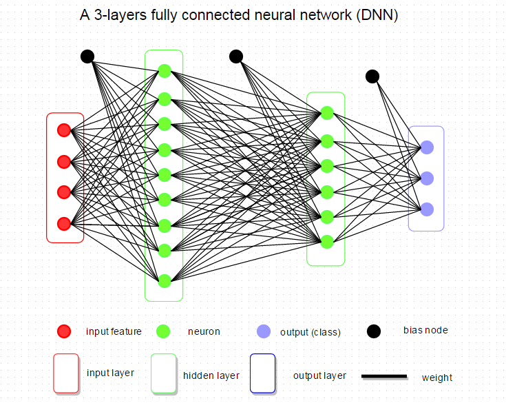Now, we will go through the basic components of DNN and show you how it is implemented in R. Weights and Bias Take above DNN architecture, for example, there are 3 groups of weights from the input layer to first hidden layer, first to second hidden layer and second hidden layer to output layer. Bias unit links to every hidden node and which affects the output scores, but without interacting with the actual data. In our R implementation, we represent weights and bias by the matrix. Weight size is defined by,

(number of neurons layer M) X (number of neurons in layer M+1)

and weights are initialized by random number from rnorm. Bias is just a one dimension matrix with the same size of neurons and set to zero. Other initialization approaches, such as calibrating the variances with 1/sqrt(n) and sparse initialization, are introduced in weight initialization part of Stanford CS231n. Pseudo R code:

weight.i <- 0.01*matrix(rnorm(layer size of (i) * layer size of (i+1)),
                        nrow=layer size of (i),
                        ncol=layer size of (i+1))
bias.i <- matrix(0, nrow=1, ncol = layer size of (i+1))

Another common implementation approach combines weights and bias together so that the dimension of input is N+1 which indicates N input features with 1 bias, as below code:

1
2
3

weight <- 0.01*matrix(rnorm((layer size of (i) +1) * layer size of (i+1)),
                            nrow=layer size of (i) +1,
                            ncol=layer size of (i+1))

Neuron A neuron is a basic unit in the DNN which is biologically inspired model of the human neuron. A single neuron performs weight and input multiplication and addition (FMA), which is as same as the linear regression in data science, and then FMA’s result is passed to the activation function. The commonly used activation functions include sigmoid, ReLu, Tanh and Maxout. In this post, I will take the rectified linear unit (ReLU) as activation function, f(x) = max(0, x). For other types of activation function, you can refer here. 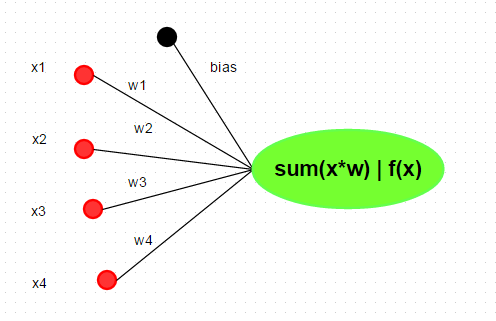In R, we can implement neuron by various methods, such as sum(xi*wi). But, more efficient representation is by matrix multiplication. R code:

1	neuron.ij <- max(0, input %*% weight + bias)

Implementation Tips _In practice, we always update all neurons in a layer with a batch of examples for performance consideration. Thus, the above code will not work correctly.

Matrix Multiplication and Addition

As below code shown, input %*% weights and bias with different dimensions and it can’t be added directly. Two solutions are provided. The first one repeats bias_ ncol _times, however, it will waste lots of memory in big data input. Therefore, the second approach is better.

# dimension: 2X2
input <- matrix(1:4, nrow=2, ncol=2)
# dimension: 2x3
weights <- matrix(1:6, nrow=2, ncol=3)
# dimension: 1*3
bias <- matrix(1:3, nrow=1, ncol=3)
# doesn't work since unmatched dimension
input %*% weights + bias
Error input %*% weights + bias : non-conformable arrays 
 
# solution 1: repeat bias aligned to 2X3 
s1 <- input %*% weights + matrix(rep(bias, each=2), ncol=3) 
 
# solution 2: sweep addition
s2 <- sweep(input %*% weights ,2, bias, '+')
 
all.equal(s1, s2)
# [1] TRUE

Element-wise max value for a matrix

Another trick in here is to replace max by pmax to get element-wise maximum value instead of a global one, and be careful of the order in pmax :)

# the original matrix
> s1
     [,1] [,2] [,3]
[1,]    8   17   26
[2,]   11   24   37
 
# max returns global maximum 
> max(0, s1)
[1] 37
 
# s1 is aligned with a scalar, so the matrix structure is lost
> pmax(0, s1)
[1]  8 11 17 24 26 37
 
# correct 
# put matrix in the first, the scalar will be recycled to match matrix structure
> pmax(s1, 0)
     [,1] [,2] [,3]
[1,]    8   17   26
[2,]   11   24   37

Layer

Input Layer

the input layer is relatively fixed with only 1 layer and the unit number is equivalent to the number of features in the input data.

Hidden layers

Hidden layers are very various and it’s the core component in DNN. But in general, more hidden layers are needed to capture desired patterns in case the problem is more complex (non-linear).

Output Layer

The unit in output layer most commonly does not have an activation because it is usually taken to represent the class scores in classification and arbitrary real-valued numbers in regression. For classification, the number of output units matches the number of categories of prediction while there is only one output node for regression.

Build Neural Network: Architecture, Prediction, and Training

Till now, we have covered the basic concepts of deep neural network and we are going to build a neural network now, which includes determining the network architecture, training network and then predict new data with the learned network. To make things simple, we use a small data set, Edgar Anderson’s Iris Data (iris) to do classification by DNN.

Network Architecture

IRIS is well-known built-in dataset in stock R for machine learning. So you can take a look at this dataset by the summary at the console directly as below.

R code:

summary(iris)
  Sepal.Length    Sepal.Width     Petal.Length    Petal.Width          Species  
 Min.   :4.300   Min.   :2.000   Min.   :1.000   Min.   :0.100   setosa    :50  
 1st Qu.:5.100   1st Qu.:2.800   1st Qu.:1.600   1st Qu.:0.300   versicolor:50  
 Median :5.800   Median :3.000   Median :4.350   Median :1.300   virginica :50  
 Mean   :5.843   Mean   :3.057   Mean   :3.758   Mean   :1.199                  
 3rd Qu.:6.400   3rd Qu.:3.300   3rd Qu.:5.100   3rd Qu.:1.800                  
 Max.   :7.900   Max.   :4.400   Max.   :6.900   Max.   :2.500

From the summary, there are four features and three categories of Species. So we can design a DNN architecture as below. 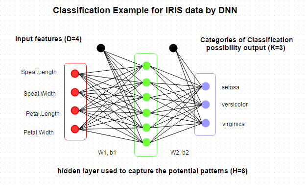And then we will keep our DNN model in a list, which can be used for retrain or prediction, as below. Actually, we can keep more interesting parameters in the model with great flexibility.

R code:

List of 7
 $ D : int 4
 $ H : num 6
 $ K : int 3
 $ W1: num [1:4, 1:6] 1.34994 1.11369 -0.57346 -1.12123 -0.00107 ...
 $ b1: num [1, 1:6] 1.336621 -0.509689 -0.000277 -0.473194 0 ...
 $ W2: num [1:6, 1:3] 1.31464 -0.92211 -0.00574 -0.82909 0.00312 ...
 $ b2: num [1, 1:3] 0.581 0.506 -1.088

Prediction Prediction, also called classification or inference in machine learning field, is concise compared with training, which walks through the network layer by layer from input to output by matrix multiplication. In output layer, the activation function doesn’t need. And for classification, the probabilities will be calculated by softmax while for regression the output represents the real value of predicted. This process is called feed forward or feed propagation.

R code:

# Prediction
predict.dnn <- function(model, data = X.test) {
  # new data, transfer to matrix
  new.data <- data.matrix(data)
 
  # Feed Forwad
  hidden.layer <- sweep(new.data %*% model$W1 ,2, model$b1, '+')
  # neurons : Rectified Linear
  hidden.layer <- pmax(hidden.layer, 0)
  score <- sweep(hidden.layer %*% model$W2, 2, model$b2, '+')
 
  # Loss Function: softmax
  score.exp <- exp(score)
  probs <-sweep(score.exp, 1, rowSums(score.exp), '/') 
 
  # select max possiblity
  labels.predicted <- max.col(probs)
  return(labels.predicted)
}

Training

Training is to search the optimization parameters (weights and bias) under the given network architecture and minimize the classification error or residuals. This process includes two parts: feed forward and back propagation. Feed forward is going through the network with input data (as prediction parts) and then compute data loss in the output layer by loss function (cost function). “Data loss measures the compatibility between a prediction (e.g. the class scores in classification) and the ground truth label.” In our example code, we selected cross-entropy function to evaluate data loss, see detail in here. After getting data loss, we need to minimize the data loss by changing the weights and bias. The very popular method is to back-propagate the loss into every layers and neuron by gradient descent or stochastic gradient descent which requires derivatives of data loss for each parameter (W1, W2, b1, b2). And back propagation will be different for different activation functions and see here and here for their derivatives formula and method, and Stanford CS231n for more training tips. In our example, the point-wise derivative for ReLu is: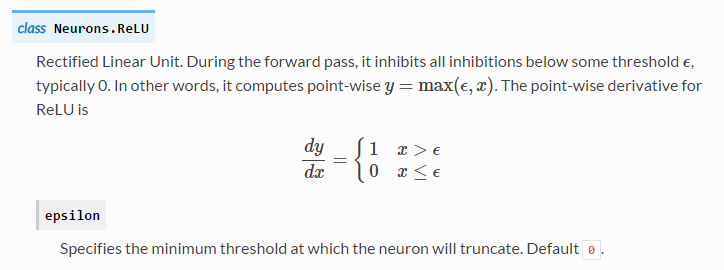

R code:

# Train: build and train a 2-layers neural network 
train.dnn <- function(x, y, traindata=data, testdata=NULL,
                  # set hidden layers and neurons
                  # currently, only support 1 hidden layer
                  hidden=c(6), 
                  # max iteration steps
                  maxit=2000,
                  # delta loss 
                  abstol=1e-2,
                  # learning rate
                  lr = 1e-2,
                  # regularization rate
                  reg = 1e-3,
                  # show results every 'display' step
                  display = 100,
                  random.seed = 1)
{
  # to make the case reproducible.
  set.seed(random.seed)
 
  # total number of training set
  N <- nrow(traindata)
 
  # extract the data and label
  # don't need atribute 
  X <- unname(data.matrix(traindata[,x]))
  Y <- traindata[,y]
  if(is.factor(Y)) { Y <- as.integer(Y) }
  # updated: 10.March.2016: create index for both row and col
  Y.len   <- length(unique(Y))
  Y.set   <- sort(unique(Y))
  Y.index <- cbind(1:N, match(Y, Y.set))
 
  # number of input features
  D <- ncol(X)
  # number of categories for classification
  K <- length(unique(Y))
  H <-  hidden
 
  # create and init weights and bias 
  W1 <- 0.01*matrix(rnorm(D*H), nrow=D, ncol=H)
  b1 <- matrix(0, nrow=1, ncol=H)
 
  W2 <- 0.01*matrix(rnorm(H*K), nrow=H, ncol=K)
  b2 <- matrix(0, nrow=1, ncol=K)
 
  # use all train data to update weights since it's a small dataset
  batchsize <- N
  # updated: March 17. 2016
  # init loss to a very big value
  loss <- 100000
 
  # Training the network
  i <- 0
  while(i < maxit && loss > abstol ) {
 
    # iteration index
    i <- i +1
 
    # forward ....
    # 1 indicate row, 2 indicate col
    hidden.layer <- sweep(X %*% W1 ,2, b1, '+')
    # neurons : ReLU
    hidden.layer <- pmax(hidden.layer, 0)
    score <- sweep(hidden.layer %*% W2, 2, b2, '+')
 
    # softmax
    score.exp <- exp(score)
    probs <-sweep(score.exp, 1, rowSums(score.exp), '/') 
 
    # compute the loss
    corect.logprobs <- -log(probs[Y.index])
    data.loss  <- sum(corect.logprobs)/batchsize
    reg.loss   <- 0.5*reg* (sum(W1*W1) + sum(W2*W2))
    loss <- data.loss + reg.loss
 
    # display results and update model
    if( i %% display == 0) {
        if(!is.null(testdata)) {
            model <- list( D = D,
                           H = H,
                           K = K,
                           # weights and bias
                           W1 = W1, 
                           b1 = b1, 
                           W2 = W2, 
                           b2 = b2)
            labs <- predict.dnn(model, testdata[,-y])      
            # updated: 10.March.2016
            accuracy <- mean(as.integer(testdata[,y]) == Y.set[labs])
            cat(i, loss, accuracy, "\n")
        } else {
            cat(i, loss, "\n")
        }
    }
 
    # backward ....
    dscores <- probs
    dscores[Y.index] <- dscores[Y.index] -1
    dscores <- dscores / batchsize
 
 
    dW2 <- t(hidden.layer) %*% dscores 
    db2 <- colSums(dscores)
 
    dhidden <- dscores %*% t(W2)
    dhidden[hidden.layer <= 0] <- 0
 
    dW1 <- t(X) %*% dhidden
    db1 <- colSums(dhidden) 
 
    # update ....
    dW2 <- dW2 + reg*W2
    dW1 <- dW1  + reg*W1
 
    W1 <- W1 - lr * dW1
    b1 <- b1 - lr * db1
 
    W2 <- W2 - lr * dW2
    b2 <- b2 - lr * db2
 
  }
 
  # final results
  # creat list to store learned parameters
  # you can add more parameters for debug and visualization
  # such as residuals, fitted.values ...
  model <- list( D = D,
                 H = H,
                 K = K,
                 # weights and bias
                 W1= W1, 
                 b1= b1, 
                 W2= W2, 
                 b2= b2)
 
  return(model)
}

Testing and Visualization

We have built the simple 2-layers DNN model and now we can test our model. First, the dataset is split into two parts for training and testing, and then use the training set to train model while testing set to measure the generalization ability of our model.

R code

########################################################################
# testing
#######################################################################
set.seed(1)
 
# 0. EDA
summary(iris)
plot(iris)
 
# 1. split data into test/train
samp <- c(sample(1:50,25), sample(51:100,25), sample(101:150,25))
 
# 2. train model
ir.model <- train.dnn(x=1:4, y=5, traindata=iris[samp,], testdata=iris[-samp,], hidden=6, maxit=2000, display=50)
 
# 3. prediction
labels.dnn <- predict.dnn(ir.model, iris[-samp, -5])
 
# 4. verify the results
table(iris[-samp,5], labels.dnn)
#          labels.dnn
#            1  2  3
#setosa     25  0  0
#versicolor  0 24  1
#virginica   0  0 25
 
#accuracy
mean(as.integer(iris[-samp, 5]) == labels.dnn)
# 0.98

The data loss in train set and the accuracy in test as below: 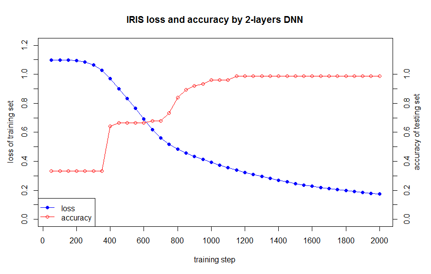Then we compare our DNN model with ‘nnet’ package as below codes.

library(nnet)
ird <- data.frame(rbind(iris3[,,1], iris3[,,2], iris3[,,3]),
                  species = factor(c(rep("s",50), rep("c", 50), rep("v", 50))))
ir.nn2 <- nnet(species ~ ., data = ird, subset = samp, size = 6, rang = 0.1,
               decay = 1e-2, maxit = 2000)
 
labels.nnet <- predict(ir.nn2, ird[-samp,], type="class")
table(ird$species[-samp], labels.nnet)
#  labels.nnet
#   c  s  v
#c 22  0  3
#s  0 25  0
#v  3  0 22
 
# accuracy
mean(ird$species[-samp] == labels.nnet)
# 0.96

Update: 4/28/2016:

Google’s tensorflow released a very cool website to visualize neural network in here. And we has taught almost all technologies as google’s website in this blog so you can build up with R as well :)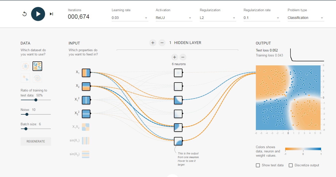

Summary

In this post, we have shown how to implement R neural network from scratch. But the code is only implemented the core concepts of DNN, and the reader can do further practices by:

Solving other classification problem, such as a toy case in here
Selecting various hidden layer size, activation function, loss function
Extending single hidden layer network to multi-hidden layers
Adjusting the network to resolve regression problems
Visualizing the network architecture, weights, and bias by R, an example in here.

In the next post, I will introduce how to accelerate this code by multicores CPU and NVIDIA GPU.

Notes: 1. The entire source code of this post in here 2. The PDF version of this post in here 3. Pretty R syntax in this blog is Created by inside-R .org (acquired by MS and dead)