Notes: 1. The entire source code of this post in here 2. The PDF version of this post in here
In previous two blogs (here and here), we illustrated several skills to build and optimize artificial neural network (ANN) with R and speed up by parallel BLAS libraries in modern hardware platform including Intel Xeon and NVIDIA GPU. Nowadays, multiple GPU accelerations are crucial for learning huge networks, one example, as Microsoft won ImageNet competition with huge network up to 1000 layers in 2015, [here and here]. In this blog, I will focus on applying CUDA implementation into our neural network offloading the computationally intensive parts into GPU and then we can easily extend CUDA implementation from single GPU to multiple GPUs under ‘parallel’ packages of R. P.S: If you want to go through all of these contents quickly, check out my presentation in GTC16 in here.
CUDA INTEGRATION
Now, we begin to introduce our ninja skills : CUDA After combined DNN code with CUDA BLAS library and several optimizations, we get the follow results in the table in the previous blog and leave one question for readers:
What is your opinion about the next step of optimizations?
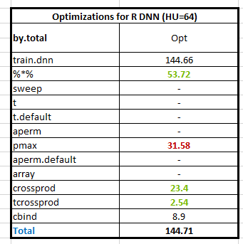
 It’s obvious that the function ‘pmax’ accounts for lots of runtimes (31.58 secs) following ‘%*%’ (53.72 secs) since ‘pmax’ is implemented by R and it will be very slow when the data size increase. (btw, you can try to increase the number of neurons in hidden layer to 1024 and profiling the code again to figure out the ratio of ‘pmax’ in the whole computation). Reviewing the functionality of ‘pmax’ in our DNN case, we implement the ReLU function and get the maximum value among input value and 0 for every neuron in hidden layer. Furthermore, because our algorithm is vectorized by matrices for high performance, the input of ‘pmax’ is a two-dimensional matrix and we can parallel maximum function into each element easily. So, let’s start to parallel the ReLu function by CUDA. I will skip the details of CUDA programming in this blog, you can refer programming guide in here. First, we can write the CUDA code to compare the input value with ZERO. Despite it is a very naïve implementation, it is still very fast than original R code. Throughout this kernel code can be executed in NVIDIA GPU, it is written by CUDA C rather than R. Next, we need to call it from R environment. In general, we have to write wrapper functions to bridge R, C/C++, and CUDA. Prof. Matloff and I have written the blog introduced linking R with CUDA step by step regarding with .Call() and .C() function with two-level wrappers from R to C/C++ and C/C++ to CUDA (here and here). A brief summary about the major difference of .C() and .Call() is shown in below table.
From the performance view, the .Call() function is selected since little overhead between R and C/C++ by avoiding explicit copying data from R to C/C++ and then from C/C++ back to R. In below code, we access data by a pointer and heavily use R internal structures with very efficient way.
1 | // difinition for R |
Next, compile the C/C++ and CUDA code together to a shared object file (.so) or dynamic link library (.dll) for loading in R.
nvcc -O3 -arch=sm_35 -G -I…/CUDA-v7.5.18/include -I…/R-3.2.0/bin/lib64/R/include/ -L…/R/lib64/R/lib –shared -Xcompiler -fPIC -o cudaR.so cudaR.cu
Finally, the CUDA version of ‘pmax’ can be called in R as simple as R builtin function with R’s wrapper, and, for infrastructure engineer, writing a nice wrapper is still an important job :)
1 | # preload static object file |
Show our performance now! By replacing ‘pmax’ with new ‘pmax.cuda’, the execution time of pmax reduces to 6.7 seconds from original 31.58 so it’s 5X speedup and totally the 1.2X speedup gains. 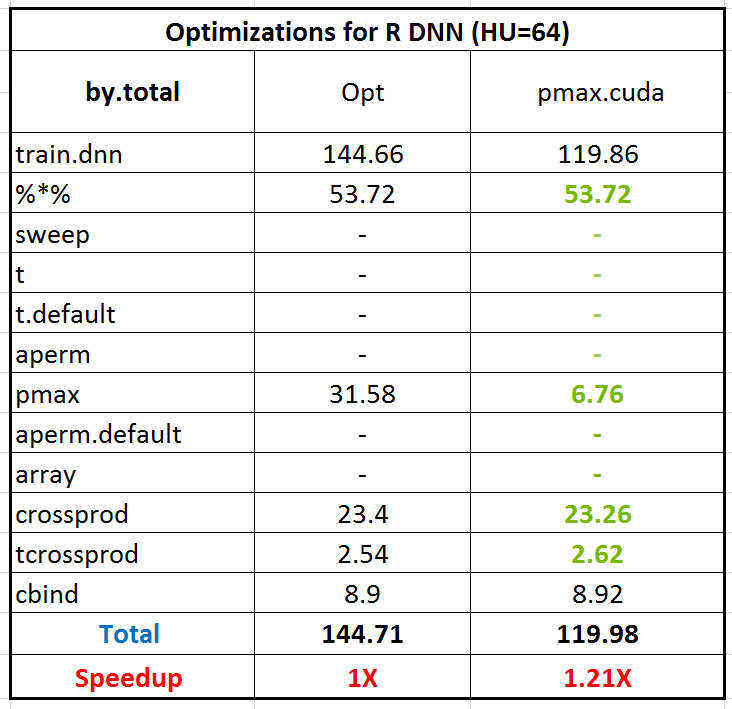
Scale out to MultiGPU
Parallel computing is not a novel concept in R community. Data scientist is familiar with parallel strategies both in speedup their model construction and inference. In fact, the requirement of parallel computing in R is even higher than C/C++. The C/C++ implementations always focus on low-level instructions and optimizations such as memory locality, communication, computation efficiency and much more while R aims to fast, easy and portability from high-level programming. Popular R packages handle most of low-level details and R users only focus on dataset decomposition and functional programming. Specifically, in this blog, we will show you parallel training of DNN with ‘parallel’ package and extend it to multiGPUs.
HOGWILD!
HOGWILD! is a data parallel model designed for stochastic gradient descent. It’s a lock-free approach with the MapReduce-like parallel-processing framework and can be used in DNN training . Thus, the training processing is designed as below: 1.Launch N workers 2.Each worker updates local weights/bias based on parts (1/N) of data 3.Master collects and averages all weights/bias from each worker 4.Each worker updates its weights/bias from master
Parallel in R
In R, this flow can be implemented by ‘multicores’ packages (currently, ‘parallel’ package includes both ‘multicores’ and ‘snow’ in CRAN). In below, flow chart is the standard workflow of ‘multicore’ packages with our DNN. ‘mclapply’ function creates two processors which shares memory by copy-on-write and each processor train the network by parts of data. After several steps, the master processor will do a reduce step to collect weights from two child processors and average them.In next iteration, two children will use the new weights. 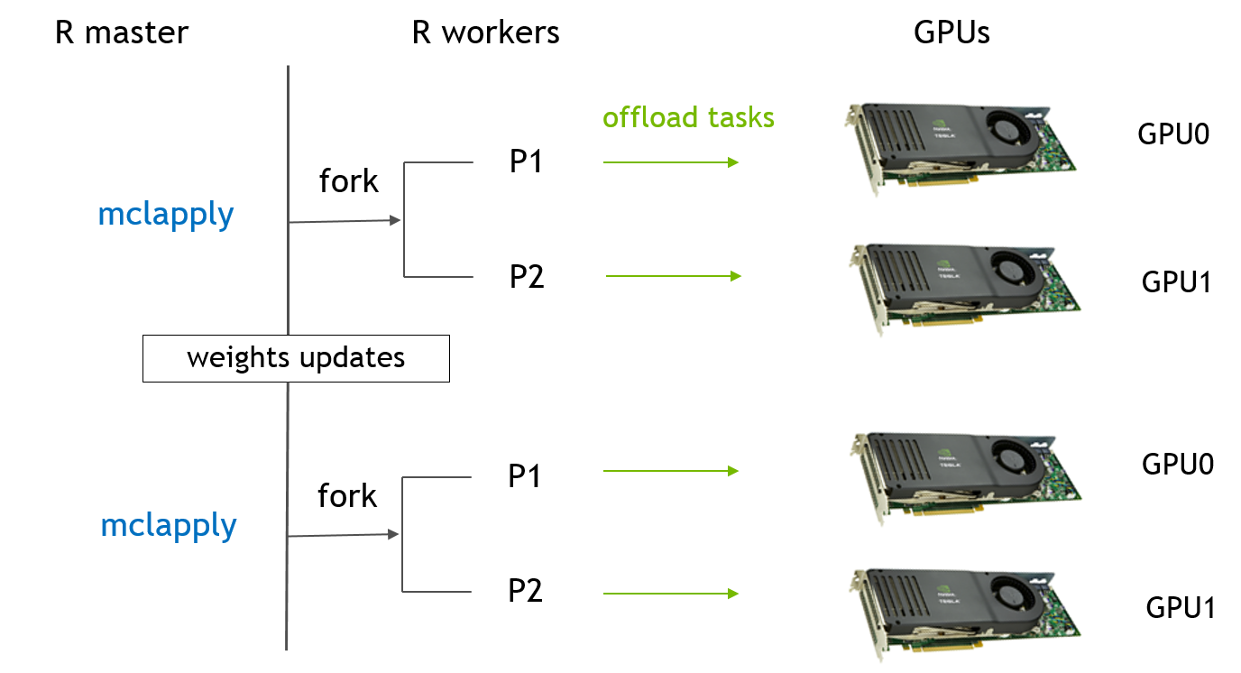 Now, let’s see the details of how R code handles this data parallel model based on below real codes . 1. ‘mclapply’ creates N (devNum) workers based on ‘mc.cores’ and each worker will execute the same function, train.dnn.cublas, with different index (1:devNum); 2. the data is divided into N (devNum) parts and each worker will load their data simultaneously by their ID then the computation, even writing, can be ideally parallelized; 3. all workers exit when ‘mclapply’ is done and the results from every worker will be saved in a list (res). Master continues to remain parts and then calculate the average of all weights and bias. 4. in the next loop, the ‘mclapply’ will use the averaged model (para.model) to train again.
1 | # Parallel Training |
Extent to MultiGPU
Then scale to multiple GPUs, the workflow is almost as similar as CPU and only different is that each worker needs to set GPU ID explicitly and then run previous CUDA accelerated code. In other words, users still are able to access the same CUDA codes that they usually use (almost) without any change! In our implementation, we adopt the strategy of a consistent one-to-one match between CPU worker with GPU by setting GPU index as below.
1 | // for multiple GPU case |
Performance Showcase
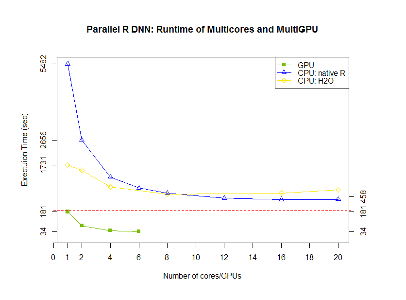
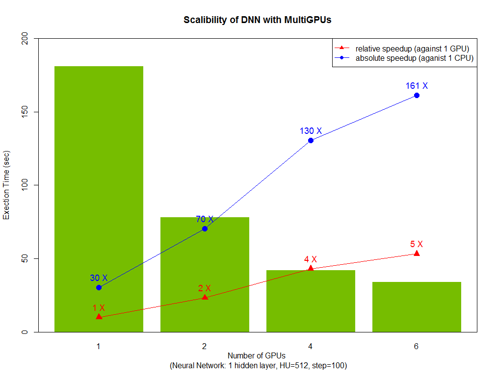
Finally, we analyzed the performance of CPU and GPU code. The line plot shows the strong scalability of native R code (1 hidden layer and 512 neurons). And compared with H2O, native R exhibits good scalability with the number of thread increase. Look at GPU parts, one thread with one GPU is faster than 20 threads CPU implementation (both native R and H2O). Next, look at GPU scalability in bar plot where 5 times speedup under 6 GPUs are reached and our algorithm achieved 160 times speedup compared with original R code. Testing on : CPU: Ivy Bridge E5-2690 v2 @ 3.00GHz, dual socket 10-core, 128G RAM; GPU: NVIDIA K40m, 12G RAM