R benchmark for High-Performance Analytics and Computing (II): GPU Packages

Posted on 2017-04-07 Edited on 2020-12-19 In GPGPU , Intel Xeon Phi

1. Overview

In the previous post (here), we have analyzed the performance gain of R in the heterogeneous system by accelerators, including NVIDIA GPU and Intel Xeon Phi. Furthermore, GPU accelerated packages can greatly improve the performance of R. Figure 1 shows the download statistics of CRAN over the years. Obviously, GPU is more and more recognized by the R community.

Figure 1 Download statistics of CRAN Package applied to the GPGPU environment over the years

2. GPU-accelerated packages

Matrix operation (BLAS) is one of the most important operations in data analysis, such as co-matrices in recommended systems and convolution calculations in deep learning. The matrix and the vector multiplication and other standard operations in R can be accelerated by GPU significantly. The most simple way to use GPU in R is through the nvBLAS (cuBLAS) library provided by NVIDIA, but other GPU accelerated packages (gputools, gmatrix, gpuR) provides a richer software and hardware interface, as shown in Table 1.

Table 1 Function comparison of the R package supported for GPGPU

2.1 Data type

Double-precision (DP) is used in nvBLAS and gputools to align with the default double precision mode of R. On the other hand, gmatrix and GPU can be more flexible for the user to choice single-precision (SP) or double-precision (DP) in the computations. And even gmatrix can support integer matrix computing. The SP computation mode can significant leverage the capability in low-mid level NVIDIA GPU cards, such as Tesla M40 and Geforce series GPUs, where the main computing power from SP floating-point operations. Therefore, this is a good news common desktop GPU users.

2.2 Data transfer

When using the GPU as a coprocessor to speed up the application, the cost of data transfer usually takes a significant portion of the time, and the size of the GPU’s built-in memory will also limit whether the application can be executed. One of the main advantages of nvBLAS is that it supports block-based data copy and calculations between CPU and GPU, so the memory required from R code can be large than built-in GPU memory. However, the host-to-device memory copy, the calculation, and the final device-to-host results are performed in a synchronized mode so that the user cannot isolate the data transfer and calculation in nvBLAS. gmatrix and gpuR provide the asynchronous mode of communication and calculation, the user can separate the data copy and the real calculation. For example, gpuR provided in the vcl * series API, it will return in the R console immediately and then R will execute the next CPU command, while GPU is computing. In this way, both CPU and GPU are working simultaneously. And we can get much more performance boost.

2.3 Programming model

Frist, nvBLAS, gmatrix are based on the CUDA programming model and it will show better performance in NVIDIA series of GPUs but the shortage is poor portability. Then, gpuR is based on OpenCL, a standard heterogeneous programming interface, and more flexible. The user program of OpenCL can be executed on much more platforms, such as CPU, GPGPU, Intel Xeon Phi and FPGA.

3. Performance Benchmark and Analysis

3.1 Test environment

The test is performed on the Ali cloud HPC platform: G2 server with NVIDIA Tesla K40m, G4 server with Tesla M40. Ali cloud HPC provides independent physical server + GPU accelerator card without virtualization overhead for computing-intensive applications. Regarding GPU equipment, K40m is designed with Kepler architecture while M40 with Maxwell architecture. The M40 targets for deep learning markets especially for training. Its SP floating-point peak performance reaches 7TFlops, but DP is only 0.2TFlops.

Table 2 Ali cloud hardware platform configuration

Table 3 List of M40 and K40m hardware parameters

Table 4 Software of test used

3.2 Performance Analysis on K40 for double precision

First, let’s compare the double-precision performance of each package on the Tesla series. We use nvblas performance as the baseline and compare the calculation time of three different sizes of matrix multiplications. In the testing code as below, we only counted the execution time of core API (% %, gemm, gpuMatMult) following depth analysis. \R code for gpuR, gmatrix, gputools and nvblas with DP calculation mode

library(gpuR)
for(i in seq(1:7)) {
  ORDER = 256*(2^i)
  A = matrix(rnorm(ORDER^2), nrow=ORDER)
  B = matrix(rnorm(ORDER^2), nrow=ORDER)
  gpuA = gpuMatrix(A, type="double")
  gpuB = gpuMatrix(B, type="double")
  cputime = system.time({gpuC = gpuA %*% gpuB})[3]
 }
  
library(gmatrix)
for(i in seq(1:7)) {
  ORDER = 256*(2^i)
  A = gmatrix(rnorm(ORDER^2),ORDER,ORDER)
  B = gmatrix(rnorm(ORDER^2),ORDER,ORDER)
  C = gmatrix(0,ORDER,ORDER)
  cputime = system.time({gmm(A,B,C)})[3]
}
 
library(gputools)
for(i in seq(1:7)) {
  ORDER = 256*(2^i)
  A = matrix(rnorm(ORDER^2), nrow=ORDER)
  B = matrix(rnorm(ORDER^2), nrow=ORDER)
  cputime = system.time({C = gpuMatMult(A, B)})[3]
}
 
# nvblas, native code + PRE_LOADED
for(i in seq(1:7)) {
  ORDER = 256*(2^i)
  A = matrix(rnorm(ORDER^2), nrow=ORDER) 
  B = matrix(rnorm(ORDER^2), nrow=ORDER) 
  cputime = system.time({C = A %*% B})[3] 
}

Figure 2 Performance of the software package with the size change

In general, nvblas, gputools and gmatrix show very similar performance, because they use cuBLAS as the backend. gpuR’s performance is relatively low and variety with input sizes, such as the 4096 matrix only achieves 20% of nvblas performance but 8192 matrices can reach ~70%. From computation pattern, gputools and gmatrix apply dgemm_sm_heavy_ldg_nn API interfaces of cuBLAS to complete the matrix calculations, and computational efficiency will be slightly higher than nvblas of the block matrix calculation mode. From memory usage, as Figure 2, nvblas is the only one able to complete the large memory (out of cores/memory) calculation. For the largest matrix 32768, GPU packages (gputools, gmatrix, gpuR) will throw an exception of memory overflow. More details In Table 5, input matrix are divided into many small pieces, and then are transmitted to the GPU for computations by nvblas.

Table 5. Analysis of memory copy times from nvprof

For gmatrix, matrix (A, B, C for C = A*B) are copied to GPU and C matrix stored in the GPU side after the calculation, involving three times host-to-device data transfer and without device-to-host transfer. For gputools matrix (A, B) are copied to GPU, the result matrix ( C ) is copied back to the host side so totally twice host-to-device and once device-to-host data transfer. Because the host-to-device data transfer is faster than device-to-host, gmatrix could get better performance than gputools as table 6 shown. Finally, we take a look at gpuR performance. The matrix calculation leverages OpenCL API that the performance is less optimized on NVIDIA GPU in table 6. GEMM compute kernel _prod_TT is much slower than gputools and gmatrix. Take 8192 for example, the calculation time of cublas API is 911.4 ms and 912.3 ms for gputools and gmatrix while OpenCL is 2172.5 ms for gpuR.

Table 6 Time overhead on GPU side at matrix size of 8192 * 8192

3.3 Performance Analysis on M40 for single precision

Single precision is quite important for data scientists but openBLAS, nvblas, and gputools use default double-precision (DP) calculation mode of R. So, it will lack competition in some hardware such as Tesla M40 where the DP performance is only 0.2T. In this parts, we will show you how to leverage SP performance in R by gmatrix and gpuR. In the blow testing, we take openBLAS performance results as the baseline. *R code of gmatrix and gpuR with SP calculation mode

library(gpuR)
for(i in seq(1:7)) {
  ORDER = 256*(2^i)
  A = matrix(rnorm(ORDER^2), nrow=ORDER)
  B = matrix(rnorm(ORDER^2), nrow=ORDER)
  gpuA = gpuMatrix(A, type="float")
  gpuB = gpuMatrix(B, type="float")
  cputime = system.time({gpuC = gpuA %*% gpuB})[3]
}
 
library(gmatrix)
for(i in seq(1:7)) {
  ORDER = 256*(2^i)
  A = gmatrix(rnorm(ORDER^2),ORDER,ORDER, type="single")
  B = gmatrix(rnorm(ORDER^2),ORDER,ORDER, type="single")
  C = gmatrix(0,ORDER,ORDER, type="single")
  cputime = system.time({
    gmm(A,B,C);
    h(C);
  })[3]
}

In Figure 3, gmatrix and gpuR with SP calculation model show a very good performance boost. For the 4096 matrix size, gmatrix is 18X faster than openBLAS and 37X faster (18.22 / 0.51) than nvblas.

Figure 3 Performance with SP mode on M40

More details in Table 7, it is obvious that the computation time of SP is much less than the calculation time of DP. The calculation time of DP is about 6000 ms (nvblas, gputools), while the calculation time of SP is only about 200 ms (gmatrix) and 500 ms (gpuR). From the memory point of view, gpuR on CPU uses SP data type and gmatrix on CPU is still DP. From Table 7, we can see that memory transfer time of gputools and gmatrix is almost same, and gpuR memory transfer time is only half of it (gmatrix 153.4 ms .vs. gpuR 77.7 ms). So, gpuR are more efficient in memory usage for SP and will good for the small size of computations. Note, gmatrix does not use MEM D2H by default. In order to compare memory transfer performance with other packages, H (C) is added into the source code to make a consistent comparison.

Table 7 SP/DP performance of each Package on the M40 with matrix size of 8192*8192

Note: GEMM kernel API on M40 is magma_lds128_dgemm_kernel.

3.4 Asynchronous Mode

For the advanced user, gpuR provides a set of asynchronous mode interface. By using asynchronous interfaces, the R program will immediately return to the CPU program side after calling the interface of vcl *, and the user can continue to perform other tasks on the CPU. When the user explicitly accesses and use vcl * data, if the calculation has not yet completed, R will continue to wait; if the calculation has been completed, users can directly use. Therefore, users can use concurrency of CPU and GPU to hide the communication and computing time on GPU. In Figure 4, we compared the computing time between gpuR in asynchronous mode and gmatrix in synchronous mode (gmatrix shows the best performance in synchronous mode testing). As figure 4 shown, the sync-API execution time increases as the computational task increases but async-API keep a very tiny cost for all input size because the async-API do not include any actual calculations and just returns immediately. So, in the best case, we can hide all GPU execution time with CPU computation with a very tiny overhead. *gpuR running code with SP in asynchronous mode

library(gpuR)
 
for(i in seq(1:7)) {
  ORDER = 256*(2^i)
  vclA_f = vclMatrix(A, nrow = ORDER, type="float")
  vclB_f = vclMatrix(B, nrow = ORDER, type="float")
  cputime = system.time({vclC_f = vclA_f %*% vclB_f})[3]
}

Figure 4. Performance comparison between gpuR in asynchronous mode and gmatrix in synchronization mode

4. Conclusions and recommendations

In this blog, we analyze the performance of the most popular GPU computing package. Each package has its own unique, but also have their own advantages and disadvantages. In practices, we need to choose according to specific needs. Based on the calculation platform, the calculation mode and the ease of use, it is recommended as follows:

nvblas is suitable for

NVIDIA GPU card
Double precision calculation
Large memory consumption of the calculation, nvblas provides a very good performance and scalability
Beginners

gputools is suitable for

NVIDIA GPU card
Double precision calculation
Easy to use, and same API interface with R
Beginners

gmatrix is suitable for

NVIDIA GPU card
Single/Double precision calculation
Multilevel BLAS interface(level 1，2，3)
More extension in GPU (colsum, sort)
Memory transfer optimization but the user needs to know where the memory is saved
Intermediate/Senior users or R developers

gpuR is suitable for

Single/Double precision calculation
Multilevel BLAS interface(level 1，2，3)
Heterogeneous systems work on most of the platforms such as AMD, Intel Xeon Phi, Intel GPUs
Asynchronous calculation mode, you can better hide the communication time
Intermediate/Senior users or R developers

Parallel Computation with R and XGBoost

Posted on 2017-01-24 Edited on 2020-12-19 In General , MultiCores

XGBoost is a comprehensive machine learning library for gradient boosting. It began from the Kaggle community for online machine learning challenges, and then maintained by the collaborative efforts from the developers in the community. It is well known for its accuracy, efficiency and flexibility for various interfaces: the computational module is implemented in C++, and currently provides interfaces for R, python, Julia and Java. Its corresponding R package, xgboost, in this sense is non-typical in terms of the design and structure. Although it is common that an R package is a wrapper of another tool, not many packages have the backend supporting many ways of parallel computation. 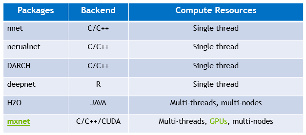The structure of the Project can be illustrated as follows: Although it is common that an R package is a wrapper of another tool, not many packages have the backend supporting many ways of parallel computation. In xgboost, most works are done in the C++ part in the above Figure. Since all interfaces share the same computational backend, there is not really a difference in terms of the accuracy or efficiency of the results from different interfaces. Users only need to prepare the data and parameters in the preferred language, then call the corresponding interface and wait for the training and prediction. This design puts most heavy works to the background, and only asks for the minimum support from each interface. For this reason, we can expect in the future there will be more languages wrapping the XGBoost backend and their users can enjoy the parallel training power. XGBoost implements a gradient boosting trees algorithm. A gradient boosting trees model trains a lot of decision trees or regression trees in a sequence, where only one tree is added to the model at a time, and every new tree depends on the previous trees. This nature limits the level of parallel computation, since we cannot build multiple trees simultaneously. Therefore, the parallel computation is introduced in a lower level, i.e. in the tree-building process at each step. Specifically, the parallel computation takes place in the operation where the model scans through all features on each internal node and set a threshold. Say we have a 4-core CPU for the training computation, then XGBoost separate the features into 4 groups. For the splitting operation on a node, XGBoost distributes the operation on each feature to their corresponding core. The training data is stored in a piece of shared memory, each core only needs to access one group of features, and perform the computation individually. The implementation is done in C++ with the help of OpenMP. It is obvious that users can benefit fully from the parallel computation if the number of features is larger than the number of threads of the CPU. XGBoost also supports training on a cluster, or with external memory. We will briefly introduce them in the following parts.

In the following part, we will demonstrate the performance of the R package with different parallel strategies. We hope this introduction can be an example of a computational efficient R package.

1. Multi-threading on a single machine

XGBoost offers the option to parallel the training process in an implicit style on a single machine, which could be a workstation or even your own laptop. This is one of the reasons that the Kaggle community loves it. In R, the switch of multi-threading computation is just a parameter nthread:

require(xgboost)
x = matrix(rnorm(100*10000), 10000, 100)
y = x %*% rnorm(100) + rnorm(1000)

system.time({
  bst = xgboost(data = x, label = y, nthread = 1, nround = 100, verbose = FALSE)
})
# ser system elapsed
# 10.98 0.05 11.06

system.time({
  bst = xgboost(data = x, label = y, nthread = 4, nround = 100, verbose = FALSE)
})
# user system elapsed
# 20.80 0.67 3.37

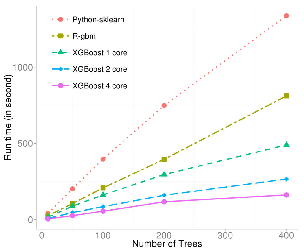In the results from the toy example, there is a noticeable difference between the one-thread and four-thread trainings. As a comparison, we made the following figure from a competition data(https://www.kaggle.com/c/higgs-boson/data) on Kaggle. The experiments were run on a laptop with an i7-4700m CPU. The marks R and python are the vanilla gradient boosting machine implementation. XGBoost is the fastest when using only one thread. By employing 4 threads the process can be almost 4x faster. To reproduce the above results, one can find related scripts at:https://github.com/dmlc/xgboost/tree/master/demo/kaggle-higgs. Note that the plot was made in 2015, thus the results may vary due to changes in the packages.

2. Parallel on a Cluster

For some cases where the size of data is too large to fit into the memory, people may set up a cluster to parallel the training process. However, a uniformed API of multi-nodes parallel computation for different interface languages is still left to be developed. The current standard way to parallel the training is to use the C++ backend with a configuration file which manages the model parameters and then submit it to Yarn. For further information, please read the official documentation: http://xgboost.readthedocs.io/en/latest/tutorials/aws_yarn.html. It is also possible to distribute the computation in one’s own cluster, but there’s no documentation provided yet. One thing worth noticing is that when performing multi-node parallel computation, the data is split by the rows, thus on each node it is (almost) impossible to search for the exact best splitting point. As a result, XGBoost switches to an approximate algorithm mentioned in this paper. Briefly speaking, the approximate algorithm creates a histogram to represent each feature based on its numerial distribution. It reduces the amount of calculation on slaves, makes the reduce step easier, and maintains the precision at the same time.

3. External Memory

External memory is a compromise of large size of input and insufficient computational resources. The basic idea is simple: store the input data on an SSD, which is cheaper than memory and faster than HDD, and repeatedly load a chunk of data into memory to train the model partially. Comparing to the parallel training on a cluster, this strategy also uses the approximate algorithm, but is more convenient to configure and call, and is also cheaper for most users. To enable the external memory for R, we need to make sure that the compiler on your machine supports it. Usually it is fine with the latest gcc/clang. For windows users with mingw, however, is not able to try it out. The data files also need to be in the libsvm format on the disk. Files used in this demo can be downloaded at https://github.com/dmlc/xgboost/tree/master/demo/data. Here’s the usual way to load the data into memory with xgboost’s own data structure:

dtrain = xgb.DMatrix('agaricus.txt.train')
# [15:57:38] 6513x127 matrix with 143286 entries loaded from agaricus.txt.train
dtest = xgb.DMatrix('agaricus.txt.test')
# [15:57:38] 1611x127 matrix with 35442 entries loaded from agaricus.txt.test

model = xgboost(data = dtrain, nround = 2, objective = "binary:logistic")
# [1] train-error:0.000614 
# [2] train-error:0.001228

Now if we add the suffix:

dtrain = xgb.DMatrix('agaricus.txt.train#train.cache')
# [15:57:45] SparsePage::Writer Finished writing to train.r0-1.cache.row.page
# [15:57:45] SparsePageSource: Finished writing to train.r0-1.cache
# [15:57:45] 6513x127 matrix with 143286 entries loaded from agaricus.txt.train#train.cache
dtest = xgb.DMatrix('agaricus.txt.test#test.cache')
# [15:57:45] SparsePage::Writer Finished writing to test.r0-1.cache.row.page
# [15:57:45] SparsePageSource: Finished writing to test.r0-1.cache
# [15:57:45] 1611x127 matrix with 35442 entries loaded from agaricus.txt.test#test.cache

model = xgboost(data = dtrain, nround = 2, objective = "binary:logistic")
# [15:57:45] SparsePage::Writer Finished writing to train.r0-1.cache.col.page
# [1] train-error:0.000614 
# [2] train-error:0.001228

Note the only difference is just the suffix: A “#” and the string following. The suffix can be arbitrary string as the prefix of the generated cache files, as printed in the output. With the suffix, the function automatically marks the file for external memory training. In the external memory mode we can also perform multi-threading training for each chunk of data, because the chunks are taken into the training process in a linear relationship. More details are included in this paper.

Summary

XGBoost puts effort in the three popular parallel computation solutions, multithreading, distributed parallel and out-of-cores computations. The idea of this project is to only expose necessary APIs for different language interface design, and hide most computational details in the backend. So far the library is fast and user-friendly, we wish it could inspire more R package developers to balance the design and efficiency. The development will be continued, and contributions on code and ideas are always welcome :)

R with Parallel Computing from User Perspectives

Posted on 2016-09-10 Edited on 2020-12-19 In Accelerators , General , GPGPU , MultiCores , Performance Optimizaiton

This article is originally published in Capital of Statistic by Chinese [link] and I would like to thank He Tong for lots of great suggestions. All code in this post can be found on GitHub [link].

Data scientists are already very familiar with statistical software like R, SAS, SPSS, MATLAB; however, some of them are relatively inexperienced in parallel computing. So, in this post, I will introduce you some basic concepts on the use of parallel computing in R.

What is Parallel Computing？

Parallel computing, specifically, should include high-performance computers and parallel software. The peak performance of high-performance computers increases quickly. In the most recent ranking of the world’s TOP500 supercomputers, Chinese Sunway Taihu Light topped the list with 93 PFLOPS (here). For most individuals, small and medium enterprises, high-performance computers are too expensive. So, the application of high-performance computers is indeed limited, mainly in the field of national defense, military, aerospace and research areas. In recent years, with the rapid developments of multicore CPU, cheap cluster, and various accelerators (NVIDIA GPU, Intel Xeon Phi, FPGA), personal computers has been comparable to high-performance computers. On the other hand, the software changes lag a lot. Imagine what software you’re using supported parallel operations, Chrome, Visual Studio or R? Software parallelization requires more research and development supports. It is called code modernization for the procedure of changing the serial code to parallel, which sounds a very interesting work. But, in practice, a large number of bug fixes, data structure rewrite, uncertain software behaviors and cross-platform issues greatly increase the software development and maintenance costs.

Why R Needs Parallel Computing?

Let’s come back to R. As one of the most popular statistical software, R has a lot of advantages, such as a wealth of statistical models, data processing tools, and powerful visualization capabilities. However, with an increasing amount of data, R’s memory usage and computation mode limit R to scale. From the memory perspective, R uses in-memory calculation mode. All data need to be processed in the main memory (RAM). Obviously, its advantages are high computational efficiency and speed, but the drawback is that the size of the problem can be handled by R is very limited (<RAM ). Secondly, R core is a single-threaded program. Thus, in the modern multi-core processors, R can not effectively use all the computing cores. If the R went to the Sunway CPU of 260 computing cores, single-threaded R only take 1/260 computing power and waste other computing cores of 259/260.

Solution？Parallel Computing!

Parallel computing technology can solve the problem that single-core and memory capacity can not meet the application needs. Thus, the parallel computing technology will be extremely expansion of the use of R. From R 2.14 (Feb 2012), ‘parallel‘ package is installed by default. Obviously, R core development team also attached great importance to parallelization.

How to Use Parallel Computing?

From the user’s view, parallel computing in R can be divided into implicit and explicit computing mode.

Implicit Mode

Implicit computing hides most of the details for the user. It is not necessary to know how to allocate hardware resources, distribute workloads and gather results. The computations will start automatically based on the current hardware resources. Obviously, this mode is the most favorable. We can achieve higher performance without changing the calculation mode and our codes. Common implicit parallel mode includes:

Using Parallel Libraries

Parallel libraries, such as Intel MKL，NVIDIA cuBLAS, OpenBLAS are usually provided by the hardware manufacturer with in-depth optimizations based on the corresponding hardwares, so its performance is hugely better than R libraries. It is recommended choosing a high-performance R library at compile time or loading by LD_PRELOAD at runtime. The details of compiling, loading and using BLAS libraries can be found in the one of our previous blog (in here). In the first diagram, the matrix calculation experiments, parallel libraries on 1 or 2 CPUs is a hundred times faster than R original library. On the second, we can see the GPU math library shows remarkable speed for some common analysis algorithms as well. Now, let’s run an interesting example in which we didn’t call GEMM function explicitly but still get lots of performance improvements from parallel BLAS library. In below example, we train MNIST dataset by DBN,deep belief network, (SRBM,Stacked Restricted Boltzmann Machine ) with deepnet package. This example refers the blog of “training MNIST data with the package deepnet“ where the author got the accuracy of 0.004% on training data and 2% on testing data. Because the original network of c(500,500,250,125) is too huge to run, I simplified the network architecture in our case and the code of deepnet_mnist.R in here.

#install.packages("data.table")
#install.packages("deepnet")
 
library(data.table)
library(deepnet)
 
# download MNIST dataset in below links
# https://h2o-public-test-data.s3.amazonaws.com/bigdata/laptop/mnist/train.csv.gz
# https://h2o-public-test-data.s3.amazonaws.com/bigdata/laptop/mnist/test.csv.gz
mnist.train <- as.matrix(fread("./train.csv", header=F))
mnist.test  <- as.matrix(fread("./test.csv", header=F))
 
# V785 is the label
x <- mnist.train[, 1:784]/255
y <- model.matrix(~as.factor(mnist.train[, 785])-1)
 
system.time(
    nn <- dbn.dnn.train(x,y,
                        hidden=c(64),
                        #hidden=c(500,500,250,125),
                        output="softmax",
                        batchsize=128, 
                        numepochs=100, 
                        learningrate = 0.1)
)

Thus, we run this piece of code twice. We got 3.7X **and **2.5Xspeedup (runtime of 2581 sec .vs. 693 sec and 1213 sec ) by Intel MKL and OpenBLAS library on Intel SandyBridge E-2670.

> R CMD BATCH deepnet_mnist.R
> cat deepnet_mnist.Rout
deep nn has been trained.
     user system   elapsed 
 2574.013  1.404  2581.882
 
> env LD_PRELOAD=/.../tools/OpenBLAS/lib/libopenblas.so R CMD BATCH deepnet_mnist.R
> cat deepnet_mnist.Rout
deep nn has been trained.
     user    system  elapsed 
 4752.005 25881.221 1213.644
 
# Compiled with Intel Compiler and MKL
> R CMD BATCH deepnet_mnist.R
> cat deepnet_mnist.Rout
deep nn has been trained.
      user  system elapsed 
 10770.641 290.486 693.146

Using MultiThreading Functions

OpenMP is a multithreading library based on shared memory architecture for application acceleration. The latest R has been opened OpenMP options (-fopenmp) at compile time on Linux, which means that some of the calculations can be run in multithreaded mode. For example , dist is implemented by multithreading with OpenMP. The example code as below (ImplicitParallel_MT.R):

# Comparison of single thread and multiple threads run
# using Internal function to set thread numbers, not very grace, but don't find a good way till now.
# Ang suggestion?
setNumThreads <- function(nums=1) {
  .Internal(setMaxNumMathThreads(nums))
  .Internal(setNumMathThreads(nums))
}
 
# dataset from 2^6 to 2^11
for(i in 6:11) {
  ORDER <- 2^i
  m <- matrix(rnorm(ORDER*ORDER),ORDER,ORDER)
  setNumThreads(1)
  res <- system.time(d <- dist(m))
  print(res)
  setNumThreads(20)
  res <- system.time(d <- dist(m))
  print(res)
}

Using Parallel Packages

In the list of R high-performance computing, there are lots of parallel packages and tools. These parallel packages can be used like any other R packages quickly and conveniently. R users can always focus on the problem itself, without having to think too much about parallelism implementations and performance issues. Take H2O.ai for example, it takes Java as the backend to achieve multi-threading and multi-nodes computing. Users only need to load the package, and then initialize H2O with thread number. After that subsequent calculations, such as GBM, GLM, DeepLearning algorithm, will automatically be assigned to multiple threads and multiple CPUs.

library(h2o)
h2o.init(nthreads = 4)
# Connection successful!
# R is connected to the H2O cluster: 
# H2O cluster uptime: 1 hours 53 minutes 
# H2O cluster version: 3.8.3.3 
# H2O cluster name: H2O_started_from_R_patricz_ywj416 
# H2O cluster total nodes: 1 
# H2O cluster total memory: 1.55 GB 
# H2O cluster total cores: 4 
# H2O cluster allowed cores: 4 
# H2O cluster healthy: TRUE 
# H2O Connection ip: localhost 
# H2O Connection port: 54321 
# H2O Connection proxy: NA 
# R Version: R version 3.3.0 (2016-05-03)

Explicit Mode

Explicit parallel computing requires the user to be able to deal with more details, including data partitions, task distributions, and final results collections. Users not only need to understand their own algorithms but also need to have a certain understanding of hardware and software stack. Thus, it’s a little difficult for users. Fortunately, parallel computing framework in R, such as parallel,Rmpi and foreach, provides the simple parallel programming approach by mapping structure. R users only need to transfer the code into the form of *apply or for, and then replace them by parallel APIs such as mc*apply or foreach. For more complex calculation flow, the user can repeat the process of map-and-reduce. Now, we show you a parallel example by solving quadratic equation with *apply and for style. The whole code in ExplicitParallel.R. First, we present a non- vectorized function for solving the equation, which can handle several special cases, such as second quadratic coefficient is zero, or second and first quadratic term are zero, or the number of the square root is negative.

# Not vectorized function
# Quadratic Equation: a*x^2 + b*x + c = 0
solve.quad.eq <- function(a, b, c) 
{
  # Not validate eqution: a and b are almost ZERO
  if(abs(a) < 1e-8 && abs(b) < 1e-8) return(c(NA, NA) )

  # Not quad equation
  if(abs(a) < 1e-8 && abs(b) > 1e-8) return(c(-c/b, NA))

  # No Solution
  if(b*b - 4*a*c < 0) return(c(NA,NA))

  # Return solutions
  x.delta <- sqrt(b*b - 4*a*c)
  x1 <- (-b + x.delta)/(2*a)
  x2 <- (-b - x.delta)/(2*a)

  return(c(x1, x2))
}

And then, we randomly generated three big vectors to storage three coefficients.

# Generate data 
len <- 1e8
a <- runif(len, -10, 10)
a[sample(len, 100,replace=TRUE)] <- 0
 
b <- runif(len, -10, 10)
c <- runif(len, -10, 10)

*apply IMPLEMENTATION:

First, we look at the serial code. The data is mapped into solver function,solve.quad.eq by lapply, and the results are saved into list finally.

# serial code
system.time(
  res1.s <- lapply(1:len, FUN = function(x) { solve.quad.eq(a[x], b[x], c[x])})
)

Next, we use the function of mcLapply (multicores) in parallel package to parallelize calculations in lapply. From the API interface, the usage of mcLapply is really similar with lapply in addition to specifying the core numbers. mcLapply creates multiple copies of the current R session based on Linux fork mechanism, and evenly assign compute tasks into multiple processes regarding with input index. Finally, the master R session will collect the results from all worker sessions. If we specify two worker processes, one process calculated 1:(len/2) while another computing (len/2+1):len, and finally two parts of results will be merged into res1.p. However, due to the use of Linux mechanisms, this version can’t be executed on Windows platform.

# parallel, Linux and MAC platform
library(parallel)
# multicores on Linux
system.time(
  res1.p <- mclapply(1:len, 
                      FUN = function(x) { solve.quad.eq(a[x], b[x], c[x]) }, 
                      mc.cores = 4)
)

For non-Linux users, we can use parLapply function in parallel package to achieve parallelism. parLapply function supports different platforms including Windows, Linux and Mac with better portability, but its usage is a little complicated than mclapply. Before using parLapply function, we need to create a computing group (cluster) first. Computing group is a software-level concept, which means how many R worker processes we need to create (Note: par*apply package will create several new R processes rather than copies of R master process from mc*apply). Theoretically, the size of the computing group is not affected by the hardware configuration.For example, we can create a group with 1000 R worker processes on any machine. In practice, we usually use the same size of computing group with hardware resources (such as physical cores) so that each worker process of R can be mapped to a physical core. In the following example, we start with detectCores function to determine the number of computing cores in the machine.It is noteworthy that detectCores() returns the number of Hyper-Threading rather than real physical cores.For example, there are two physical cores on my laptop, and each core can simulate two hyperthreading , so detectCores() return value is 4. However, for many compute-intensive tasks, the Hyper-Threading is not much helpful for improving performance, so we use the parameter of logical=FALSE to get the actual number of physical cores and then create the same number group.Since the worker processes in the group is new R sessions, the data and functions of the parent process is not visible. Therefore, we have to broadcast the data and functions to all worker processes by clusterExport function. Finally parLapply will distribute the tasks to all R worker processes evenly, and then gather results back.

# cluster on Windows
cores <- detectCores(logical = FALSE)
cl <- makeCluster(cores)
clusterExport(cl, c('solve.quad.eq', 'a', 'b', 'c'))
system.time(
  res1.p <- parLapply(cl, 1:len, function(x) { solve.quad.eq(a[x], b[x], c[x]) })
)
stopCluster(cl)

for IMPLEMENTATION:

The computation approach of for is very similar with *apply. In the following serial implementation, we created a matrix for storage results and update the results one by one in the inner loop.

# for style: serial code
res2.s <- matrix(0, nrow=len, ncol = 2)
system.time(
  for(i in 1:len) {
      res2.s[i,] <- solve.quad.eq(a[i], b[i], c[i])
  }
)

For the for loop parallelization, we can use %dopar% in foreach package to distribute the computations to multiple R workers. foreach package provides a method of data mapping, but does not include the establishment of computing group.Therefore, we need to create a computing group by doParallel or doMC package. Creating computing group is as same as before, except setting backend of computations by registerDoParallel. Now we consider the data decomposition. Actually, we want each R worker process to deal with continuous computing tasks. Suppose we have two R worker processes, the process 1 computes from 1:len/2, another process for (len/2+1):len. Therefore, in the following example code, we evenly distribute the vectors to computing group and each process calculates the size of chunk.size. Another important skill is using local matrix to save partial results in each process. Last, combine local results together by .combine='rbind' parameter.

# foreach, work on Linux/Windows/Mac
library(foreach)
library(doParallel)
 
# Real physical cores in my computer
cores <- detectCores(logical = FALSE)
cl <- makeCluster(cores)
registerDoParallel(cl, cores=cores)
 
# clusterSplit are very convience to split data but it takes lots of extra memory
# chunks <- clusterSplit(cl, 1:len)
 
# split data by ourselves
chunk.size <- len/cores
 
system.time(
  res2.p <- foreach(i=1:cores, .combine='rbind') %dopar%
  { 
    # local data for results
    res <- matrix(0, nrow=chunk.size, ncol=2)
    for(x in ((i-1)*chunk.size+1):(i*chunk.size)) {
        res[x - (i-1)*chunk.size,] <- solve.quad.eq(a[x], b[x], c[x])
    }
    # return local results
    res
  }
)
 
stopImplicitCluster()
stopCluster(cl)

Finally, we tested the code on Linux platform with 4 threads and can gain more than **3X speedup ** for every parallel implementation!

Challenges and Prospects

Challenges :In practice, the problem needed to be resolved by parallel computing is not such simple as our examples. To parallelize R and its eco-system are still very difficult because,

R is a decentralized and non-commercial software

R is not developed by a compact organization or company while most of R’s packages are contributed by users. It means that it is difficult to adjust and unify software architecture and design with the same philosophy. On the other hand, commercial software, such as Matlab, with unified development, maintenance, and management, can be relatively easier to restructure and reconstruct. Therefore, after several times update, the parallelism of commercial software will be much higher.

The infrastructure design of R is still single-threaded

R was originally designed for single-threaded so that many of the underlying data structures and functions are not thread-safe. Therefore, lots of codes need to be rewritten or adjust for high-level parallel algorithms. But it likely will destroy the original design patterns.

The packages are highly dependent

Assume that we use package B in R, and B depends on some functions of package A. If package B is improved by multithreading first; after that package A is also enhanced by parallelization. So, it is likely to appear hybrid parallel when we use package B. It may lead lots of strange errors (BUGs) and performance decrease if there is no comprehensive design and testing during developments. Prospects: How will the future of parallelism in R ?

High-performance components from commercial and research organizations

Essentially, software developments are inseparable from the human and financial investments. The packages, such as H2O, MXNet, Intel DAAL, improve the performance significantly from parallelism with long-term supports.

Cloud Platform

With the rise of cloud computing ,Data Analyst as a Services (DAAS) and Machine Learning as a Service (MLAS) are more and more popular.The major cloud providers optimize their tools, including R, from hardware deployments, database, high-level algorithms and explore much more parallelism in application level. For example, Microsoft recently launched a series supports for R in their cloud (here). Therefore, parallel in R will be more transparent. The user does the same things in R, but the real computing will be distributed to the cloud.

R and openMP: boosting compiled code on multi-core cpu-s

Posted on 2016-07-26 Edited on 2020-12-19 In Accelerators , MultiCores , Vectorization

Introduction

Sometimes you just need more speed. And sometime plain R does not provide it. This article is about boosting your R code with C++ and openMP. OpenMP is a parallel processing framework for shared memory systems. This is an excellent way to use all the cpu cores that are sitting, and often just idling, in any modern desktop and laptop. Below, I will take a simple, even trivial problem—ML estimation of normal distribution parameters—and solve it first in R, thereafter I write the likelihood function in standard single-threaded C++, and finally in parallel using C++ and openMP. Obviously, there are easier ways to find sample mean and variance but this is not the point. Read it, and try to write your own openMP program that does something useful!

R for Simplicity

Assume we have a sample of random normals and let’s estimate the parameters (mean and standard deviation) by Maximum Likelihood (ML). We start with pure R. The log-likelihood function may look like this:

llR <- function(par, x) {
  mu <- par[1]
  sigma <- par[2]
  sum(-1/2*log(2*pi) - log(sigma) - 1/2*((x - mu)^2)/sigma^2)
}

Note that this code is fully vectorized ((x-mu) is written with no explicit loop) and hence very fast. Obviously, this is a trivial example, but it is easy to understand and parallelize. Now generate some data

1	x <- rnorm(1e6)

and start values, a bit off to give the computer more work:

1	start <- c(1,1)

Estimate it (using maxLik package):

library(maxLik)
system.time(m <- maxLik(llR, start=start, x=x))

# user system elapsed
# 2.740  0.184   2.931

summary(m)

# --------------------------------------------
# Maximum Likelihood estimation
# Newton-Raphson maximisation, 6 iterations
# Return code 2: successive function values within tolerance limit
# Log-Likelihood: -1419125
# 2 free parameters
# Estimates:
# Estimate Std. error t value Pr(> t)
# [1,] 0.0010318 0.0010001 1.032 0.302
# [2,] 1.0001867 0.0007072 1414.236 <2e-16 ***
# ---
# Signif. codes: 0 ‘***’ 0.001 ‘**’ 0.01 ‘*’ 0.05 ‘.’ 0.1 ‘ ’ 1
# --------------------------------------------

The code runs 2.6s on an i5-2450M laptop using a single cpu core. First, let’s squeeze more out of the R code. Despite being vectorized, the function can be improved by moving the repeated calculations out of the (vectorized) loop. We can re-write it as:

llROpt <- function(par, x) {
  mu <- par[1]
  sigma <- par[2]
  N <- length(x)
  -N*(0.5*log(2*pi) + log(sigma)) - 0.5*sum((x - mu)^2)/sigma^2
}

Now only (x - mu)^2 is computed as vectors. Run it:

library(maxLik)
system.time(m <- maxLik(llROpt, start=start, x=x))

# user  system elapsed
# 0.816   0.000   0.818

You see—just a simple optimization gave a more than three–fold speed improvement! I don’t report the results any more, as those are virtually identical.

C for Speed

Now let’s implement the same function in C++. R itself is written in C, however there is an excellent library, Rcpp, that makes integrating R and C++ code very easy. It is beyond the scope of this post to teach readers C and explain the differences between C and C++. But remember that Rcpp (and hence C++) offers a substantially easier interface for exchanging data between R and compiled code than the default R API. Let’s save the log-likelihood function in file loglik.cpp. It might look like this:

#include <cmath>
#include <Rcpp.h>
  
using namespace Rcpp;
  
RcppExport SEXP loglik(SEXP s_beta, SEXP s_x) {
  NumericVector x(s_x);
  NumericVector beta(s_beta);
  // make Rcpp vector out of R SEXP
  double mu = beta[0];
  // first element is 0 in C++
  double sigma = beta[1];
  double ll = 0;
  for(int i = 0; i < x.length(); i++) {
      ll -= (x[i] - mu)*(x[i] - mu);
  }
  ll *= 0.5/sigma/sigma;
  ll -= (0.5*log(2*M_PI) + log(sigma))*x.length();
  NumericVector result(1, ll);
  // create 'numeric' vector of length 1, filled with
  // ll values
  return result;
}

The function takes two parameters, s_beta and s_x. These are passed as R general vectors, denoted SEXP in C. As SEXP-s are complicated to handle, the following two lines transform those to ‘NumericVector’s, essentially equivalent to R ‘numeric()’. The following code is easy to understand. We loop over all iterations and add (x[i] - mu)^2. Loops are cheap in C++. Afterwards, we add the constant terms only once. Note that unlike R, indices in C++ start from zero. This program must be compiled first. Normally the command

1	R CMD SHLIB loglik.cpp

takes care of all the R-specific dependencies, and if everything goes well, it results in the DLL file. Rcpp requires additional include files which must be specified when compiling, the location of which can be queried with Rcpp:::CxxFlags() command in R, or as a bash one-liner, one may compile with

1	PKG_CXXFLAGS=$(echo 'Rcpp:::CxxFlags()'\| R --vanilla --slave) R CMD SHLIB loglik.cpp

Now we have to create the R-side of the log-likelihood function. It may look like this:

llc <- function(par, x) {
  library(Rcpp)
  dyn.load("loglik.so") # extension '.so' is platform-specific!
  res <- .Call("loglik", par, x)
  res
}

It takes arguments ‘par’ and ‘x’, and passes these down to the DLL. Before we can invoke (.Call) the compiled code, we must load the DLL. You may need to adjust the exact name according to your platform here. Note also that I haven’t introduced any security checks neither at the R nor the C++ side. This is a quick recipe for crashing your session, but let’s avoid it here in order to keep the code simple. Now let’s run it:

system.time(m <- maxLik(llc, start=start, x=x))

# user  system elapsed
# 0.896   0.020   0.913

The C code runs almost exactly as fast as the optimized R. In case of well vectorized computations, there seems to be little scope for improving the speed by switching to C.

Parallelizing the code on multicore CPUs

Now it is time to write a parallel version of the program. Take the C++ version as the point of departure and re-write it like this:

#include <cmath>
#include <Rcpp.h>
#include <omp.h>
  
using namespace Rcpp;
  
RcppExport SEXP loglik_MP(SEXP s_beta, SEXP s_x, SEXP s_nCpu) {
    NumericVector x(s_x);
    NumericVector beta(s_beta);
    int n_cpu = IntegerVector(s_nCpu)[0];
    double mu = beta[0];
    double sigma = beta[1];
    double ll = 0;
    omp_set_dynamic(0);         // Explicitly disable dynamic teams
    omp_set_num_threads(n_cpu); // Use n_cpu threads for all
                                // consecutive parallel regions
#pragma omp parallel
    {
        double ll_thread = 0;
#pragma omp for 
        for(int i = 0; i < x.length(); i++) {
            ll_thread -= (x[i] - mu)*(x[i] - mu);
        }
#pragma omp critical
        {
            ll += ll_thread;
        }
    }
    ll *= 0.5/sigma/sigma;
    ll -= (0.5*log(2*M_PI) + log(sigma))*x.length();
    NumericVector result(1, ll);
    return result;
}

The code structure is rather similar to the previous example. The most notable novelties are the ‘#pragma omp’ directives. These tell the compiler to insert parallelized code here. Not all compilers understand it, and others may need special flags, such as -fopenmp in case of gcc, to enable openMP support. Otherwise, gcc just happily ignores the directives and you will get a single-threaded application. The likelihood function also includes the argument _n_Cpu_, and the commands omp_set_dynamic(0) and omp_set_num_threads(n_cpu). This allows to manipulate the number of threads explicitly, it is usually not necessary in the production code. For compiling the program, we can add -fopenmp to our one-liner above:

1	PKG_CXXFLAGS="$(echo 'Rcpp:::CxxFlags()'\| R --vanilla --slave) -fopenmp" R CMD SHLIB loglikMP.cpp

assuming it was saved in “loglikMP.cpp”. But now you should seriously consider writing a makefile instead. We use three openMP directives here:

#pragma omp parallel
{
/* code block */
}

This is the most important omp directive. It forces the code block to be run in multiple threads, by all threads simultaneously. In particular, variable _ll_thread_ is declared in all threads separately and is thus a thread-specific variable. As OMP is a shared-memory parallel framework, all data declared before #pragma omp parallel is accessible by all threads. This is very convenient as long as we only read it. The last directive is closely related:

#pragma omp critical
{
/* code block */
}

This denotes a piece of threaded code that must be run by only one thread simultaneously. In the example above all threads execute ll += ll_thread, but only one at a time, waiting for the previous thread to finish if necessary. This is because now we are writing to shared memory: variable ll is defined before we split the code into threads. Allowing multiple threads to simultaneously write in the same shared variable almost always leads to trouble. Finally,

1 2	#pragma omp for for(...) { /* code block */ }

splits the for loop between threads in a way that each thread will only go through a fraction of the full loop. For instance, in our case the full loop goes over 1M observations, but in case of 8 threads, each will receive only 125k. As the compiler has to generate code for this type of loop sharing, parallel loops are less flexible than ordinary single-threaded loops. For many data types, summing the thread–specific values we did with #pragma omp critical can be achieved directly in the loop by specifying #pragma omp parallel for reduction(+:ll) instead. As all the parallel work is done at C level, the R code remains essentially unchanged. We may write the corresponding loglik function as

llcMP <- function(par, nCpu=1, x) {
  library(Rcpp)
  dyn.load("loglikMP.so")
  res <- .Call("loglik_MP", par, x, as.integer(nCpu))
  res
}

How fast is this?

1
2
3

system.time(m <- maxLik(llcMP, start=start, nCpu=4, x=x))
# user  system elapsed
# 0.732   0.016   0.203

On 2-core/4-thread cpu, we got a more than four–fold speed boost. This is impressive, given the cpu does have 2 complete cores only. Obviously, the performance improvement depends on the task. This particular problem is embarrasingly parallel, the threads can work completely independent of each other.

Timing Examples

As an extended timing example, we run all the (optimized) examples above using a Xeon-L5420 cpu with 8 cores, single thread per core. The figure below depicts the compute time for single-threaded R and C++ code, and for C++/openMP code with 8 threads, as a function of data size. The figure reveals several facts. First, for non-parallelized code we can see that

Optimized R and C++ code are of virtually identical speed.
compute time grows linearily in data size.

For openMP code the figure tells

openMP with 8 threads is substantially slower for data size less than about 100k. For larger data, multi-threaded approach is clearly faster.
openMP execution time is almost constant for data size up to 4M. For larger data vectors, it increases linearily. This suggests that for smaller data size, openMP execution time is dominated by thread creation and management overheads, not by computations.

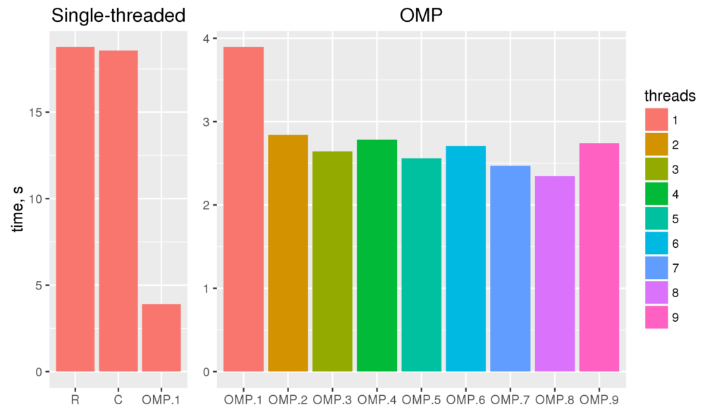Finally, let’s compare the computation times for different number of threads for 8M data size. The figure shows the run time for single threaded versions of the code (R and C), and multi-threaded openMP versions with 1 to 9 threads (OMP.1 to OMP.9).

More cpus give us shorter execution times. 1-thread OMP will run almost 1.7 times slower than 8-threaded version (3.9 and 2.3 s respectively).
The gain of more cpu cores working on the problem levels off quickly. Little noticeable gain is visible for more than 3 cores. It indicates that the calculations are only partly limited by computing-power. Another major bottleneck may be memory speed.
Last, and most strikingly, even the single threaded OMP version of the code is 4.8 times faster than single-threaded C++ version with no OMP (18.6 and 3.9 s respectively)! This is a feature of the particular task, the compiler and the processor architecture. OMP parallel for–loops allow the compiler to deduce that the loops are in fact independent, and use faster SSE instruction set. This substantially boosts the speed but requires more memory bandwidth.

Conclusion

With the examples above I wanted to show that for many tasks, openMP is not hard to use. If you know some C++, parallelizing your code may be quite easy. True, the examples above are easy to parallelize at R-level as well, but there are many tasks where this is not true. Obviously, in the text above I just scratched the surface of openMP. If you consider using it, there are many excellent sources on the web. Take a look!

I am grateful to Peng Zhao for explaining the parallel loops and SSE instruction set.

R for Deep Learning (III): CUDA and MultiGPUs Acceleration

Posted on 2016-05-09 Edited on 2020-12-19 In Accelerators , GPGPU , Performance Optimizaiton

Notes: 1. The entire source code of this post in here 2. The PDF version of this post in here

In previous two blogs (here and here), we illustrated several skills to build and optimize artificial neural network (ANN) with R and speed up by parallel BLAS libraries in modern hardware platform including Intel Xeon and NVIDIA GPU. Nowadays, multiple GPU accelerations are crucial for learning huge networks, one example, as Microsoft won ImageNet competition with huge network up to 1000 layers in 2015, [here and here]. In this blog, I will focus on applying CUDA implementation into our neural network offloading the computationally intensive parts into GPU and then we can easily extend CUDA implementation from single GPU to multiple GPUs under ‘parallel’ packages of R. P.S: If you want to go through all of these contents quickly, check out my presentation in GTC16 in here.

CUDA INTEGRATION

Now, we begin to introduce our ninja skills : CUDA After combined DNN code with CUDA BLAS library and several optimizations, we get the follow results in the table in the previous blog and leave one question for readers:

What is your opinion about the next step of optimizations?

It’s obvious that the function ‘pmax’ accounts for lots of runtimes (31.58 secs) following ‘%*%’ (53.72 secs) since ‘pmax’ is implemented by R and it will be very slow when the data size increase. (btw, you can try to increase the number of neurons in hidden layer to 1024 and profiling the code again to figure out the ratio of ‘pmax’ in the whole computation). Reviewing the functionality of ‘pmax’ in our DNN case, we implement the ReLU function and get the maximum value among input value and 0 for every neuron in hidden layer. Furthermore, because our algorithm is vectorized by matrices for high performance, the input of ‘pmax’ is a two-dimensional matrix and we can parallel maximum function into each element easily. So, let’s start to parallel the ReLu function by CUDA. I will skip the details of CUDA programming in this blog, you can refer programming guide in here. First, we can write the CUDA code to compare the input value with ZERO. Despite it is a very naïve implementation, it is still very fast than original R code. Throughout this kernel code can be executed in NVIDIA GPU, it is written by CUDA C rather than R. Next, we need to call it from R environment. In general, we have to write wrapper functions to bridge R, C/C++, and CUDA. Prof. Matloff and I have written the blog introduced linking R with CUDA step by step regarding with .Call() and .C() function with two-level wrappers from R to C/C++ and C/C++ to CUDA (here and here). A brief summary about the major difference of .C() and .Call() is shown in below table.

From the performance view, the .Call() function is selected since little overhead between R and C/C++ by avoiding explicit copying data from R to C/C++ and then from C/C++ back to R. In below code, we access data by a pointer and heavily use R internal structures with very efficient way.

// difinition for R
extern "C" {
   SEXP pmax_cuda(SEXP A, SEXP threshold, SEXP devID);
}
 
//CUDA: simple implementation of pmax
__global__ void pmax_kernel(double *A, 
                            const int M, 
                            const int N, 
                            const double threshold)
{
  int tid = blockIdx.x * blockDim.x + threadIdx.x;
  if(tid &lt; M*N) { A[tid] = (A[tid]&gt;threshold)?A[tid]:0;
  }
  return;
}
 
// Wrapper code between R and CUDA 
SEXP pmax_cuda(SEXP A, SEXP threshold, SEXP devID)
{
   // data structure for GPU
   double *A_host = NULL;
   double *A_d = NULL;
   double gw = 0;
   int mm = 0, nn = 0;
   int gpuID = 0;
  
   // data transfer from R to C by pointers
   A_host = REAL(A);
   SEXP Rdim = getAttrib(A, R_DimSymbol);
   mm = INTEGER(Rdim)[0];
   nn = INTEGER(Rdim)[1];
   gw = REAL(threshold)[0];
   gpuID = INTEGER(devID)[0];
 
   // for multiple GPU case 
   cudaSetDevice(gpuID);
  
   // return value, allocated in C and can be used in R directly
   SEXP Rval;
   PROTECT(Rval = allocVector(REALSXP, mm*nn));
 
   // GPU memory allocation
   cudaMalloc(&amp;A_d, mm*nn*sizeof(double));
   if(NULL == A_d) {
     printf("\nNo RAM space in GPU!\n");
     UNPROTECT(1);
     return R_NilValue;
   }
  
   // memory copy from CPU to GPU
   cudaMemcpy(A_d, A_host, mm*nn*sizeof(double), cudaMemcpyHostToDevice); 
  
   // CUDA: pmax, really computation parts
   pmax_kernel&lt;&lt;&lt;(mm*nn-1)/512+1, 512&gt;&gt;&gt;(A_d, mm, nn, gw);
   cudaMemcpy(REAL(Rval), A_d, mm*nn*sizeof(double), cudaMemcpyDeviceToHost); 
   cudaDeviceSynchronize();
 
   // Free unused memory of GPU
   if(A_d) {cudaFree(A_d); A_d=NULL;}
 
   UNPROTECT(1);
   return Rval;
}

Next, compile the C/C++ and CUDA code together to a shared object file (.so) or dynamic link library (.dll) for loading in R.

nvcc -O3 -arch=sm_35 -G -I…/CUDA-v7.5.18/include -I…/R-3.2.0/bin/lib64/R/include/ -L…/R/lib64/R/lib –shared -Xcompiler -fPIC -o cudaR.so cudaR.cu

Finally, the CUDA version of ‘pmax’ can be called in R as simple as R builtin function with R’s wrapper, and, for infrastructure engineer, writing a nice wrapper is still an important job :)

# preload static object file
dyn.load("cudaR.so")
 
# GPU version of pmax
pmax.cuda <- function(A, threshold, devID=0L)
{
  rst <- .Call("pmax_cuda",
                A,
                threshold,
                as.integer(devID)
	      )
  dim(rst) <- dim(A)
  return(rst)
}

Show our performance now! By replacing ‘pmax’ with new ‘pmax.cuda’, the execution time of pmax reduces to 6.7 seconds from original 31.58 so it’s 5X speedup and totally the 1.2X speedup gains.

Scale out to MultiGPU

Parallel computing is not a novel concept in R community. Data scientist is familiar with parallel strategies both in speedup their model construction and inference. In fact, the requirement of parallel computing in R is even higher than C/C++. The C/C++ implementations always focus on low-level instructions and optimizations such as memory locality, communication, computation efficiency and much more while R aims to fast, easy and portability from high-level programming. Popular R packages handle most of low-level details and R users only focus on dataset decomposition and functional programming. Specifically, in this blog, we will show you parallel training of DNN with ‘parallel’ package and extend it to multiGPUs.

HOGWILD!

HOGWILD! is a data parallel model designed for stochastic gradient descent. It’s a lock-free approach with the MapReduce-like parallel-processing framework and can be used in DNN training . Thus, the training processing is designed as below: 1.Launch N workers 2.Each worker updates local weights/bias based on parts (1/N) of data 3.Master collects and averages all weights/bias from each worker 4.Each worker updates its weights/bias from master

Parallel in R

In R, this flow can be implemented by ‘multicores’ packages (currently, ‘parallel’ package includes both ‘multicores’ and ‘snow’ in CRAN). In below, flow chart is the standard workflow of ‘multicore’ packages with our DNN. ‘mclapply’ function creates two processors which shares memory by copy-on-write and each processor train the network by parts of data. After several steps, the master processor will do a reduce step to collect weights from two child processors and average them.In next iteration, two children will use the new weights. Now, let’s see the details of how R code handles this data parallel model based on below real codes . 1. ‘mclapply’ creates N (devNum) workers based on ‘mc.cores’ and each worker will execute the same function, train.dnn.cublas, with different index (1:devNum); 2. the data is divided into N (devNum) parts and each worker will load their data simultaneously by their ID then the computation, even writing, can be ideally parallelized; 3. all workers exit when ‘mclapply’ is done and the results from every worker will be saved in a list (res). Master continues to remain parts and then calculate the average of all weights and bias. 4. in the next loop, the ‘mclapply’ will use the averaged model (para.model) to train again.

# Parallel Training
res <- mclapply(1:devNum, function(id) { train.dnn.cublas(x, y, 
                                         omodel=para.model,
                                         taindata=traindata[N.start[id]:N.end[id],],
                                         devType=“GPU”, devID=(id-1), . . .) },
                mc.cores=devNum, 
                mc.preschedule=TRUE)
 
# Construct new model with parallel weights
D <- res[[1]]$D
H <- res[[1]]$H
K <- res[[1]]$K
for(i in 2:devNum) {
        res[[1]]$W1 <- res[[1]]$W1 + res[[i]]$W1
        res[[1]]$W2 <- res[[1]]$W2 + res[[i]]$W2
        res[[1]]$b1 <- res[[1]]$b1 + res[[i]]$b1
        res[[1]]$b2 <- res[[1]]$b2 + res[[i]]$b2
}

para.model <- list( D = D,
                    H = H,
                    K = K,
                    # weights and bias
                    W1= res[[1]]$W1/devNum, 
                    b1= res[[1]]$b1/devNum, 
                    W2= res[[1]]$W2/devNum, 
                    b2= res[[1]]$b2/devNum)

Extent to MultiGPU

Then scale to multiple GPUs, the workflow is almost as similar as CPU and only different is that each worker needs to set GPU ID explicitly and then run previous CUDA accelerated code. In other words, users still are able to access the same CUDA codes that they usually use (almost) without any change! In our implementation, we adopt the strategy of a consistent one-to-one match between CPU worker with GPU by setting GPU index as below.

1 2	// for multiple GPU case cudaSetDevice(gpuID);

Performance Showcase

Finally, we analyzed the performance of CPU and GPU code. The line plot shows the strong scalability of native R code (1 hidden layer and 512 neurons). And compared with H2O, native R exhibits good scalability with the number of thread increase. Look at GPU parts, one thread with one GPU is faster than 20 threads CPU implementation (both native R and H2O). Next, look at GPU scalability in bar plot where 5 times speedup under 6 GPUs are reached and our algorithm achieved 160 times speedup compared with original R code. Testing on : CPU: Ivy Bridge E5-2690 v2 @ 3.00GHz, dual socket 10-core, 128G RAM; GPU: NVIDIA K40m, 12G RAM

R - GPU Programming for All with 'gpuR'

Posted on 2016-05-04 Edited on 2020-12-19 In GPGPU , MultiCores , Performance Optimizaiton

Introduction

GPUs (Graphic Processing Units) have become much more popular in recent years for computationally intensive calculations. Despite these gains, the use of this hardware has been very limited in the R programming language. Although possible, the prospect of programming in either OpenCL or CUDA is difficult for many programmers unaccustomed to working with such a low-level interface. Creating bindings for R’s high-level programming that abstracts away the complex GPU code would make using GPUs far more accessible to R users. This is the core idea behind the gpuR package. There are three novel aspects of gpuR:

Applicable on ‘ALL’ GPUs
Abstracts away CUDA/OpenCL code to easily incorporate in to existing R algorithms
Separates copy/compute functions to allow objects to persist on GPU

Broad application:

The ‘gpuR’ package was created to bring the power of GPU computing to any R user with a GPU device. Although there are a handful of packages that provide some GPU capability (e.g. gputools, cudaBayesreg, HiPLARM, HiPLARb, and gmatrix) all are strictly limited to NVIDIA GPUs. As such, a backend that is based upon OpenCL would allow all users to benefit from GPU hardware. The ‘gpuR’ package therefore utilizes the ViennaCL linear algebra library which contains auto-tuned OpenCL kernels (among others) that can be leveraged for GPUs. The headers have been conveniently repackaged in the RViennaCL package. It also allows for a CUDA backend for those with NVIDIA GPUs that may see further improved performance (contained within the companion gpuRcuda package not yet formally released).

Abstract away GPU code:

The gpuR package uses the S4 object oriented system to have explicit classes and methods that all the user to simply cast their matrix or vector and continue programming in R as normal. For example:

ORDER = 1024
 
A = matrix(rnorm(ORDER^2), nrow=ORDER)
B = matrix(rnorm(ORDER^2), nrow=ORDER)
gpuA = gpuMatrix(A, type="double")
gpuB = gpuMatrix(B, type="double")
 
C = A %*% B
gpuC = gpuA %*% gpuB
 
all.equal(C == gpuC[])
[1] TRUE

The gpuMatrix object points to a matrix in RAM which is then computed by the GPU when a desired function is called. This avoids R’s habit of copying the memory of objects. For example:

library(pryr)
 
# Initially points to same object
x = matrix(rnorm(16), 4)
y = x
 
address(x)
[1] "0x16177f28"
 
address(y)
[1] "0x16177f28"
 
# But once modify the second object it creates a copy
y[1,1] = 0
 
address(x)
[1] "0x16177f28"
 
address(y)
[1] "0x15fbb1d8

In contrast, the same syntax for a gpuMatrix will modify the original object in-place without any copy.

library(pryr)
library(gpuR)
 
# Initially points to same object
x = gpuMatrix(rnorm(16), 4, 4)
y = x
 
x@address
[1] <pointer: 0x6baa040>
 
y@address
[1] <pointer: 0x6baa040>
 
# Modification affects both objects without copy
y[1,1] = 0
 
x@address
[1] <pointer: 0x6baa040>
 
y@address
[1] <pointer: 0x6baa040>

Each new variable assigned to this object will only copy the pointer thereby making the program more memory efficient. However, the gpuMatrix> class does still require allocating GPU memory and copying data to device for each function call. The most commonly used methods have been overloaded such as %*%, +, -, *, /, crossprod, tcrossprod, and trig functions among others. In this way, an R user can create these objects and leverage GPU resources without the need to know a bunch more functions that would break existing algorithms.

Distinct Copy/Compute Functionality:

For the gpuMatix and gpuVector classes there are companion vclMatrix and vclVector class that point to objects that persist in the GPU RAM. In this way, the user explicitly decides when data needs to be moved back to the host. By avoiding unnecessary data transfer between host and device performance can significantly improve. For example:

vclA = vclMatrix(rnorm(10000), nrow = 100)
vclB = vclMatrix(rnorm(10000), nrow = 100)
vclC = vclMatrix(rnorm(10000), nrow = 100)
 
# GEMM
vclD = vclA %*% vclB
 
# Element-wise addition
vclD = vclD + vclC

In this code, the three initial matrices already exist in the GPU memory so no data transfer takes place in the GEMM call. Furthermore, the returned matrix remains in the GPU memory. In this case, the ‘vclD’ object is still in GPU RAM. As such, the element-wise addition call also happens directly on the GPU with no data transfers. It is worth also noting that the user can still modify elements, rows, or columns with the exact same syntax as a normal R matrix.

1
2
3

vclD[1,1] = 42
vclD[,2] = rep(12, 100)
vclD[3,] = rep(23, 100)

These operations simply copy the new elements to the GPU and modify the object in-place within the GPU memory. The ‘vclD’ object is never copied to the host.

Benchmarks:

With all that in mind, how does gpuR perform? Here are some general benchmarks of the popular GEMM operation. I currently only have access to a single NVIDIA GeForce GTX 970 for these simulations. Users should expect to see differences with high performance GPUs (e.g. AMD FirePro, NVIDIA Tesla, etc.). Speedup relative to CPU will also vary depending upon user hardware.

(1) Default dGEMM vs Base R

R is known to only support two numeric types (integer and double). As such, Figure 1 shows the fold speedup achieved by using the gpuMatrix and vclMatrix classes. Since R is already known to not be the fastest language, an implementation with the OpenBLAS backend is included as well for reference using a 4 core Intel i5-2500 CPU @ 3.30GHz. As can be seen there is a dramatic speedup from just using OpenBLAS or the gpuMatrix class (essentially equivalent). Of interest is the impact of the transfer time from host-device-host that is typical in many GPU implementations. This cost is eliminated by using the vclMatrix class which continues to scale with matrix size. 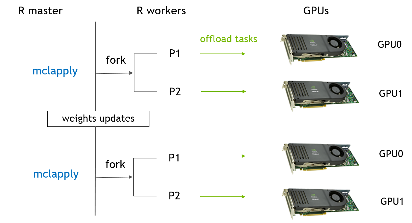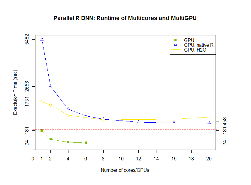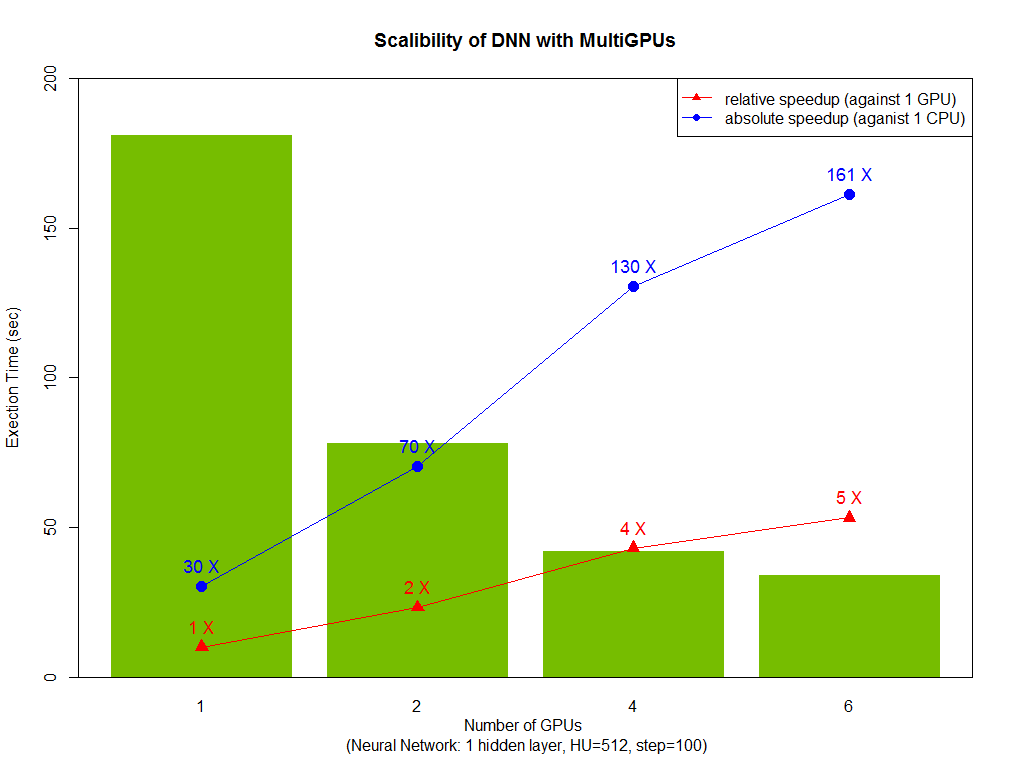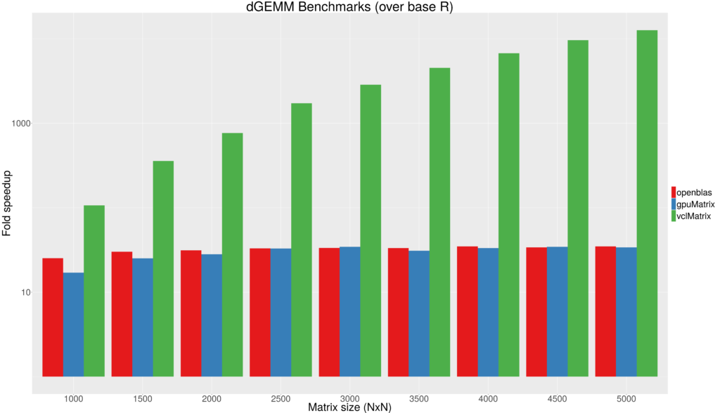[caption id=”attachment_768” align=”aligncenter” width=”640”] Figure 1 - Fold speedup achieved using openblas (CPU) as well as the gpuMatrix/vclMatrix (GPU) classes provided in gpuR.[/caption]

(2) sGEMM vs Base R

In many GPU benchmarks there is often float operations measured as well. As noted above, R does not provide this by default. One way to go around this is to use the RcppArmadillo or RcppEigen packages and explicitly casting R objects as float types. The armadillo library will also default to using the BLAS backend provided (i.e. OpenBLAS). Float types are implemented gpuR by setting type = "float" in the matrix calls (e.g. vclMatrix(mat, type = "float")) in Figure 2 shows the impact of using float data types. OpenBLAS continues to provide a noticeable speedup but gpuMatrix begins to outperform once matrix order exceeds 1500. The vclMatrix continues to demonstrate the value in retaining objects in GPU memory and avoiding memory transfers. 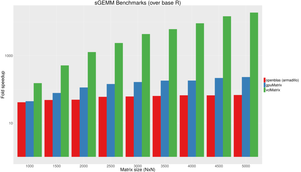[caption id=”attachment_769” align=”aligncenter” width=”640”] Figure 2 - Float type GEMM comparisons. Fold speedup achieved using openblas (via RcppArmadillo) as well as the gpuMatrix/vclMatrix (GPU) classes provided in gpuR.[/caption] To give an additional view on the performance achieved by 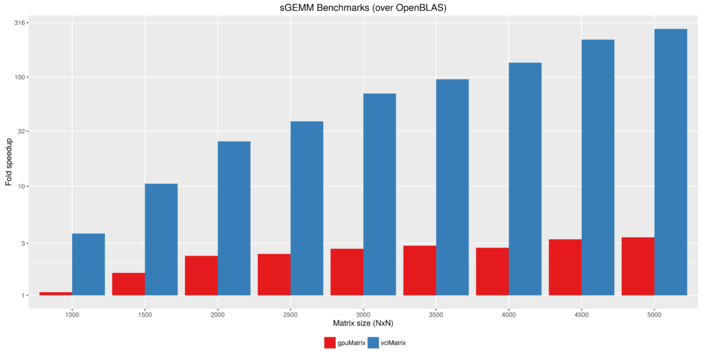gpuMatrix and vclMatrix is comparing directly against the OpenBLAS performance. The gpuMatrix reaches ~2-3 fold speedup over OpenBLAS whereas vclMatrix scales to over 100 fold speedup! It is curious as to why the performance with vclMatrix is so much faster (only differing in host-device-host transfers). Further optimization with gpuMatrix will need to be explored (fresh eyes are welcome) accepting limitations in the BUS transfer speed. Performance will certainly improve with improved hardware capabilities such as NVIDIA’s NVLink. [caption id=”attachment_831” align=”aligncenter” width=”737”] Figure 3 - Fold speedup achieved over openblas (via RcppArmadillo) float type GEMM comparisons vs the gpuMatrix/vclMatrix (GPU) classes provided in gpuR.[/caption]

Conclusion

The gpuR package has been created to bring GPU computing to as many R users as possible. It is the intention to use gpuR to more easily supplement current and future algorithms that could benefit from GPU acceleration. The gpuR package is currently available on CRAN. The development version can be found on my github in addition to existing issues and wiki pages (assisting primarily in installation). Future developments include solvers (e.g. QR, SVD, cholesky, etc.), scaling across multiple GPUs, ‘sparse’ class objects, and custom OpenCL kernels. As noted above, this package is intended to be used with a multitude of hardware and operating systems (it has been tested on Windows, Mac, and multiple Linux flavors). I only have access to a limited set of hardware (I can’t access every GPU, let along the most expensive). As such, the development of gpuR depends upon the R user community. Volunteers who possess different hardware are always welcomed and encouraged to submit issues regarding any discovered bugs. I have begun a gitter account for users to report on successful usage with alternate hardware. Suggestions and general conversation about gpuR is welcome.

R benchmark for High-Performance Analytics and Computing (I):Accelerators

Posted on 2016-04-15 Edited on 2020-12-19 In Accelerators , GPGPU , MultiCores

Objectives of Experiments

R is more and more popular in various fields, including the high-performance analytics and computing (HPAC) fields. Nowadays, the architecture of HPC system can be classified as pure CPU system, CPU + Accelerators (GPGPU/FPGA) heterogeneous system, CPU + Coprocessors system. In software side, high performance scientific libraries, such as basic linear algebra subprograms (BLAS), will significantly influence the performance of R for HPAC applications. So, in the first post of R benchmark series, the experiments mainly contain two aspects: (1) Performance on different architectures of HPC system, (2) Performance on different BLAS libraries.

Benchmark and Testing Goals

In this post, we choose R-25 benchmark (available in here ) which includes the most popular, widely acknowledged functions in the high performance analytic field. The testing script includes fifteen common computational intensive tasks (in Table-1) grouped into three categories: (1) Matrix Calculation (1-5) (2) Matrix function (6-10) (3) Programmation (11-15)

Table-1 R-25 Benchmark Description

Task Number

R-25 Benchmark Description

1 Creation,transposition,deformation of a 2500*2500 matrix

2 2400*2400 normal distributed random matrix

3 Sorting of 7,000,000 random values

4 2800*2800 cross-product matrix

5 Linear regression over a 3000*3000 matrix

6 FFT over 2,400,000 random values

7 Eigenvalues of a 640*640 random values

8 Determinant of a 2500*2500 random matrix

9 Cholesky decomposition of a 3000*3000 matrix

10 Inverse of a 1600*1600 random matrix

11 3,500,000 Fibonacci numbers calculation(vector calculation)

12 Creation of a 3000*3000 Hilbert matrix(matrix calculation)

13 Grand common divisors of 400,000 pairs(recursion)

14 Creation of a 500*500 Toeplitz matrix(loops)

15 Escoufier’s method on a 45*45 matrix(mixed)

In our benchmark, we measured the performance of R-25 benchmark on various hardware platforms, including Intel Xeon CPU processors, NVIDIA GPGPU cards and Intel Xeon Phi coprocessors. Meanwhile, R built with different BLAS libraries results in different performance, so we tested R with self-contained BLAS, OpenBLAS, Intel MKL and CUDA BLAS. Because the performance of self-contained BLAS is hugely** lower than the other BLAS library and in practice HPAC users of R always built R with high performance BLAS, the testing results running with self-contained BLAS is negligible. ** Moreover, in order to investigate the performance of functions or algorithms such as GEMM that HPC users mostly used, we explore the speed-up when varying the size of the matrices and number of elements as known as scalability.

System Descriptions

To evaluate the applicability of different methods for improving R performance in a HPC environment, the hardware and software of platform we used listed in the Table-2 and Table-3.

Results and Discussions

(1) General Comparisons

Fig. 1 shows the speedup of R using different BLAS libraries and different hosts. The default R running with OpenBLAS is shown in red as our baseline for comparison so that its speedup is constantly equal to one. Intel Xeon E5-2670 has eight physical cores in one chipset, so there are 16 physical cores in one server node.Intel MKL library supports the single thread mode (Sequential) or OpenMP threading mode. MKL with OpenMP threading mode defaultly uses all physical cores in one node(here is 16).Fig.1 shows the results of using Intel MKL for 1 thread and 16 threads with automatic parallel execution are shown in blue. There are five subtasks showing a significant benefit from either optimized sequential math library or the automatic parallelization with MKL including crossprod (matrix size 2800*2800), linear regression, matrix decomposition, computing inverse and determinant of a matrix. Other non-computational intensive tasks received very little performance gains from parallel execution with MKL.

Fig.1 Performance comparison among Intel MKL and NVIDIA BLAS against R+OpenBLAS

We also exploited parallelism with CUDA BLAS (libnvblas.so) on NVIDIA GPU platform. Since drop-in library (nvblas) only accelerated the level 3 BLAS functions and overhead of preloading, the result (green column) in Fig.2 showed little benefit and even worse performance for some computing tasks against Intel MKL accelerations.

Fig.2 Performance comparison for CPU and GPU with NVIDIA BLAS and Intel MKL

(2) Scalability on NVIDIA GPU

The performance using two GPU devices (green column) is not superior to using one GPU device (blue column) , even the results of some subtasks on one GPU device gains more. Taking the function crossproduct with computing-intensive as an example is to explain the difference between one GPU device and two GPU device, as followed the Fig. 3. The advantage of the performance of the two card is gradually displayed as the size of the matrix increases. The sub-vertical axis shows the ratio of the elapsed time on two devices to one device. A ratio greater than 1 indicates that the two card performance is better than 1 cards,and the greater the ratio of the two cards, the better the performance of the card.

Fig.3 Scalability for 1X and 2X NVIDIA K40m GPU for ‘crossprod’ function

(3) Heterogeneous Parallel Models on Intel Xeon Phi (MIC)

To compare the parallelism supported by pure CPU (Intel Xeon processor) and Intel Xeon Phi coprocessor, we conducted batch runs ( 10 times for the average elapsed time) with the different matrix size of matrix production. MKL supports automatic offload computation to Intel Xeon Phi card, but before using you must know , Automatic offload functions in MKL

Level-3 BLAS: GEMM, TRSM, TRMM, SYMM
LAPACK 3 amigos : LU, QR, Cholesky

Matrix size for offloading

GEMM: M, N >2048, K>256
SYMM: M, N >2048
TRSM/TRMM: M, N >3072
LU: M, N>8192

Here, we use **a%*%a** substituted for the function `crossprod` used in R-benchmark-25.R because _crossprod_ can not be auto-offloaded to Intel Xeon Phi. We compared the elapsed time running on CPU+Xeon Phi with running on pure CPU. In Fig.4, the vertical axis is the ratio of running elapsed time with CPU+Xeon Phi running mode to elapsed time with pure CPU running mode. The results showed the greater size of the matrix, the better performance CPU+Xeon Phi gains. The matrix size less than 4000 could get the best performance on pure CPU.

Fig.4 Heterogeneous Computing with Intel Xeon and Intel Xeon Phi

Fig.5 shows the 80% computation on Xeon Phi could get the best performance as the matrix size is growing, 70% computation on Xeon Phi could get the steadily better performance when the matrix size larger than 2000.

Fig.5 Different computation ratio on Intel Xeon Phi result in different performance

(4) Comparison NVIDIA GPU with Intel Xeon Phi

Here, we plotted the results of NVIDIA GPU and Intel Xeon Phi compared to Intel Xeon in Fig.6. In general, 80% running on Xeon Phi(2X 7110P)+Xeon CPU(2X E5-2670) gets similar performance to 1X K40m+2X E5-2670(2X 7110P ~ 1X K40m). When the matrix size is less than 12000, GPU gets better performance than Xeon Phi. And after that, Intel Xeon Phi shows the similar performance with NVIDIA K40m. For this benchmark, it can clearly seen that NVIDIA’s Tesla GPU(2X K40m) outperforms significantly.At 16000 of matrix size, nearly 3.9x faster than the 8-core dual E5-2670(Sandy-Bridge CPU) and 2.3x faster than the 80% running on Xeon Phi. The Xeon Phi is 2.8x faster than the Sandy-Bridge.

Fig.6 Comparison NVIDIA GPU with Intel Xeon Phi

Conclusions

In this article, we tested the R-benchmark-25.R script on the different hardware platform with different BLAS libraries. From our analysis, we concluded (1) R built with Intel MKL (either sequential or threaded) can accelerate lots of computationally intensive algorithms of HPAC and get the best performance, such as linear regression, PCA, SVD (2) R is performed faster on GPU for matrix production (GEMM) since it’s really computational intensive algorithm and GPU has more computing cores than Intel Xeon or Xeon Phi (3) R executed in the heterogeneous platforms (CPU+GPU or CPU+MIC) can gain more performance improvements (4) R can get more benefits from multiple GPUs, especially for large GEMM operations. In the next post, we will further investigate the benchmark performance with different R parallel packages and commercial productions of R .

Appendix : How to build R with different BLAS library

STOCK R

(1) Stock R build

Download base R package from the R project website, the current package is R-3.2.3.

Enter into the R root directory, and execute

$./configure –with-readline=no –with-x=no –prefix=$HOME/R-3.2.3-ori

$make -j4

$make install

(2) Add R bin directory and library directory to the environment variables PATH and LD_LIBRARY_PATH seperately, just like as:

export PATH=$HOME/R-3.2.3-ori/bin:$PATH

export LD_LIBRARY_PATH=$HOME/R-3.2.3-ori/lib64/R/lib:$LD_LIBRARY_PATH

R WITH OPENBLAS

(1) OpenBLAS build

Download OpenBlas-0.2.15.tar.gz from http://www.openblas.net/

Change directory to OpenBLAS Home directory, and execute

$make

$make PREFIX=$OPENBLAS_INSTALL_DIRECTORY install

(2) Set the OpenBLAS library environment

(3) Run benchmark

$LD_PRELOAD=$OPENBLAS_HOME/lib/libopenblas.so R

R WITH INTEL MKL

(1）Obtain Intel parallel studio software from Intel website

(2) Install the parallel studio

(3) Set the Intel compiler and MKL library environment

(4) Build R with MKL

Link MKL libraries configuration file mkl.conf as follows:

a. Sequencial MKL or MKL single thread

#make sure intel compiler is installed and loaded which can be set in .bashrc

as e.g.

source /opt/intel/bin/compilervars.sh intel64
MKL_LIB_PATH=/opt/intel/mkl/lib/intel64## Use intel compiler
CC=’icc -std=c99′
CFLAGS=’-g -O3 -wd188 -ip ‘F77=’ifort’
FFLAGS=’-g -O3 ‘CXX=’icpc’
CXXFLAGS=’-g -O3 ‘FC=’ifort’
FCFLAGS=’-g -O3 ‘## MKL sequential, ICC
MKL=” -L${MKL_LIB_PATH}
-Wl,–start-group
-lmkl_intel_lp64
-lmkl_sequential
-lmkl_core
-Wl,–end-group”
b. OpenMP Threading MKL

#make sure intel compiler is installed and loaded which can be set in .bashrc

as e.g.

source /opt/intel/bin/compilervars.sh intel64
MKL_LIB_PATH=/opt/intel/mkl/lib/intel64## Use intel compiler
CC=’icc -std=c99′
CFLAGS=’-g -O3 -wd188 -ip ‘F77=’ifort’
FFLAGS=’-g -O3 ‘CXX=’icpc’
CXXFLAGS=’-g -O3 ‘FC=’ifort’
FCFLAGS=’-g -O3 ‘## MKL With Intel MP threaded , ICC
MKL=” -L${MKL_LIB_PATH}
-Wl,–start-group
-lmkl_intel_lp64
-lmkl_intel_thread
-lmkl_core
-Wl,–end-group
-liomp5 -lpthread”
build R with following command,

$./configure –prefix=$HOME/R-3.2.3-mkl-icc –with-readline=no –with-x=no –with-blas=”$MKL” –with-lapack CC=’icc -std=c99′ CFLAGS=’-g -O3 -wd188 -ip ‘ F77=’ifort’ FFLAGS=’-g -O3 ‘ CXX=’icpc’ CXXFLAGS=’-g -O3 ‘ FC=’ifort’ FCFLAGS=’-g -O3 ‘

$make -j 4; make install

(5) Set $HOME/R-3.2.3-mkl-icc environment

R WITH CUDA BLAS
(1) Install the driver and CUDA tools with version up to 6.5 for NVIDIA Tesla Cards

(2)Set the CUDA environment

(3)Edit the nvblas.conf file

# This is the configuration file to use NVBLAS Library
# Setup the environment variable NVBLAS_CONFIG_FILE to specify your own config file.
# By default, if NVBLAS_CONFIG_FILE is not defined,
# NVBLAS Library will try to open the file “nvblas.conf” in its current directory
# Example : NVBLAS_CONFIG_FILE /home/cuda_user/my_nvblas.conf
# The config file should have restricted write permissions accesses# Specify which output log file (default is stderr)
NVBLAS_LOGFILE nvblas.log#Put here the CPU BLAS fallback Library of your choice
#It is strongly advised to use full path to describe the location of the CPU Library
NVBLAS_CPU_BLAS_LIB /opt/R-3.2.3-ori/lib64/R/lib/libRblas.so
#NVBLAS_CPU_BLAS_LIB &lt;mkl_path_installtion&gt;/libmkl_rt.so# List of GPU devices Id to participate to the computation
# Use ALL if you want all your GPUs to contribute
# Use ALL0, if you want all your GPUs of the same type as device 0 to contribute
# However, NVBLAS consider that all GPU have the same performance and PCI bandwidth
# By default if no GPU are listed, only device 0 will be used#NVBLAS_GPU_LIST 0 2 4
#NVBLAS_GPU_LIST ALL
NVBLAS_GPU_LIST ALL# Tile Dimension
NVBLAS_TILE_DIM 2048# Autopin Memory
NVBLAS_AUTOPIN_MEM_ENABLED#List of BLAS routines that are prevented from running on GPU (use for debugging purpose
# The current list of BLAS routines supported by NVBLAS are
# GEMM, SYRK, HERK, TRSM, TRMM, SYMM, HEMM, SYR2K, HER2K#NVBLAS_GPU_DISABLED_SGEMM
#NVBLAS_GPU_DISABLED_DGEMM
#NVBLAS_GPU_DISABLED_CGEMM
#NVBLAS_GPU_DISABLED_ZGEMM# Computation can be optionally hybridized between CPU and GPU
# By default, GPU-supported BLAS routines are ran fully on GPU
# The option NVBLAS_CPU_RATIO_&lt;BLAS_ROUTINE&gt; give the ratio [0,1]
# of the amount of computation that should be done on CPU
# CAUTION : this option should be used wisely because it can actually
# significantly reduced the overall performance if too much work is given to CPU#NVBLAS_CPU_RATIO_CGEMM 0.07

Set NVBLAS_CONFIG_FILE to the nvblas.conf location

(4) Run the benchmark

LD_PRELOAD=/opt/cuda-7.5/lib64/libnvblas.so R

R WITH MKL ON INTEL XEON PHI

(1) Build R with MKL

Build R with MKL is same to Threaded MKL at 6

(2) Enable MKL MIC Automatic Offload Mode

export MKL_MIC_ENABLE=1

export MIC_KMP_AFFINITY=compact

Otherwise , you can set the workload division between host CPU and MIC card. If one host has two MIC cards, you could set:

export MKL_HOST_WORKDIVISION=0.2

export MKL_MIC_0_WORKDIVISION=0.4

export MKL_MIC_1_WORKDIVISION=0.4

R for Deep Learning (II): Achieve High-Performance DNN with Parallel Acceleration

Posted on 2016-03-08 Edited on 2020-12-19 In GPGPU , MultiCores , Performance Optimizaiton

I would like to thank Jun Ma and all other technical reviewers and readers for their informative comments and suggestions in this post.

50 years of Data Science, David Donoho, 2015

**Computing with Data.**Every data scientist should know and use several languages for data analysis and data processing. These can include popular languages like R and Python … Beyond basic knowledge of languages, data scientists need to keep current on new idioms for efficiently using those languages and need to understand the deeper issues associated with computational efficiency.

In the previous post, R for deep learning (I), I introduced the core components of neural networks and illustrated how to implement it from scratch by R. Now, I will focus on computational performance and efficiency of R’s implementation, especially for the parallel algorithm on multicores CPU and NVIDIA GPU architectures.

Performance Profiling

In this post, we are going to a little big dataset, MNIST, for performance analysis. MNIST widely used to measure the accuracy of classification by handwritten digits in machine learning field, and also used for the competition in Kaggle (data in download page or here). Yann has provided the classification results based on various machine learning algorithms on his page.

Picture.1 Handwritten Digits in MNIST dataset

The MNIST database contains 60,000 training images and 10,000 testing images. Each of image is represented by 28*28 points so totally 784 points. In this post, I will train the neural network with 784 points as input features and the number of 0-9 as output classes, then compare the runtime of our R DNN code with H2O deep learning implementations for 2-layers networks of the various number of hidden units (HU).

# h2o
library(h2o)
# single thread
h2o.init()
 
 
train_file <- "https://h2o-public-test-data.s3.amazonaws.com/bigdata/laptop/mnist/train.csv.gz"
test_file <- "https://h2o-public-test-data.s3.amazonaws.com/bigdata/laptop/mnist/test.csv.gz"
 
train <- h2o.importFile(train_file)
test  <- h2o.importFile(test_file)
 
# To see a brief summary of the data, run the following command
summary(train)
summary(test)
 
y <- "C785"
x <- setdiff(names(train), y)
 
# We encode the response column as categorical for multinomial
#classification
train[,y] <- as.factor(train[,y])
test[,y]  <- as.factor(test[,y])
 
# Train a Deep Learning model and valid
system.time(
  model_cv <- h2o.deeplearning(x = x,
                               y = y,
                               training_frame = train,
                               distribution = "multinomial",
                               activation = "Rectifier",
                               hidden = c(32),
                               l1 = 1e-5,
                               epochs = 200)
)

As I know, H2O is the fast and most popular deep learning package in R platform implemented by Java in the backend. Thus, it will be valuable to know how much performance gap between native R code and the mature package. As below barplot shown, the hidden units of 32, 64 and 128 are tested in 200 steps. Obviously, the R DNN is significantly slow than H2O, and the runtime increases with the number of hidden units quickly. For more details, we break down the R DNN runtime into each function call by Rprof() and summaryRprof() which report out the final results including 4 parts: total.time, total.pct, self.time and self.pct. The self.time and self.pct columns represent the elapsed time for each function, excluding the time from its inner called functions. The total.time and total.pct columns mean the total elapsed time for each function including the time spent on function calls [Aloysius Lim]. From the profiling results, we can see the top 1 time-consuming function is *“%%”** which represents matrix multiplications and usually people call it GEMM (GEneral Matrix Multiplication).

> Rprof()
> mnist.model <- train.dnn(x=1:784, y=785, traindata=train, hidden=64, maxit=200, display=50)
> Rprof(NULL)
> summaryRprof()
$by.self
                   self.time self.pct total.time total.pct
"%*%"                1250.08    90.19    1250.08     90.19
"t.default"            61.62     4.45      61.62      4.45
"pmax"                 24.40     1.76      28.42      2.05
"aperm.default"        11.60     0.84      11.60      0.84
"array"                10.36     0.75      10.36      0.75
"train.dnn"             9.74     0.70    1386.00    100.00
"<="                    5.72     0.41       5.72      0.41
"mostattributes<-"      4.02     0.29       4.02      0.29
"exp"                   3.60     0.26       3.60      0.26
"sweep"                 1.58     0.11     676.32     48.80
"is.data.frame"         1.28     0.09       1.28      0.09
"colSums"               0.86     0.06       0.86      0.06
"/"                     0.52     0.04       0.52      0.04
"rowSums"               0.36     0.03       0.36      0.03
"unname"                0.18     0.01       1.46      0.11
"-"                     0.04     0.00       0.04      0.00
"t"                     0.02     0.00      61.64      4.45
"sum"                   0.02     0.00       0.02      0.00
 
$by.total
                   total.time total.pct self.time self.pct
"train.dnn"           1386.00    100.00      9.74     0.70
"%*%"                 1250.08     90.19   1250.08    90.19
"sweep"                676.32     48.80      1.58     0.11
"t"                     61.64      4.45      0.02     0.00
"t.default"             61.62      4.45     61.62     4.45
"pmax"                  28.42      2.05     24.40     1.76
"aperm"                 21.96      1.58      0.00     0.00
"aperm.default"         11.60      0.84     11.60     0.84
"array"                 10.36      0.75     10.36     0.75
"<="                     5.72      0.41      5.72     0.41
"mostattributes<-"       4.02      0.29      4.02     0.29
"exp"                    3.60      0.26      3.60     0.26
"unname"                 1.46      0.11      0.18     0.01
"is.data.frame"          1.28      0.09      1.28     0.09
"data.matrix"            1.28      0.09      0.00     0.00
"colSums"                0.86      0.06      0.86     0.06
"/"                      0.52      0.04      0.52     0.04

Parallel Acceleration

From above analysis, the matrix multiplication (“%*%”) accounts for about 90% computation time in the training stage of the neural network. Thus, the key of DNN acceleration is to speed up matrix multiplication. Fortunately, there are already several parallel libraries for matrix multiplication and we can deploy it to R easily. In this post, I will introduce three basic linear algebra subprograms (BLAS) libraries, openBLAS, Intel MKL, and cuBLAS. (In another blog, moreover, we show their performance on modern hardware architectures and instructions of installation). The former two are multithread accelerated libraries which need to be built with R together (instructions in here and here). On the other hand, it is indeed easy to apply NVIDIA cuBLAS library in R on Linux system by the drop-on wrap, nvBLAS, which can be preloaded into R in order to hijack original Rblas.so. By this way, we can leverage NVIDIA GPU’s power into R with zero programming efforts :) The below picture shows the architecture of R with BLAS libraries. Typically, R will call their own BLAS, Rblas.so,on Linux system which handles all kinds of linear algebra functions (here), but it is a single thread implementation. The trick to speed up the linear algebra calculations is to update the R standard BLAS to modern multithread libraries. For R developers, there is almost a ‘free lunch’ without rewriting their codes for parallel accelerations. As below code shown, we tested prebuilt R with openBLAS, Intel MKL and nvBLAS for 2-layers neural network of 32, 64 and 128 neurons.From the below bar chart, the runtime of R DNN are dramatically decreased and it is nearly 2X faster than H2O and 9X speedup (from 2816 to 365 for 128 hidden neurons network) than original R code!

# you must create a configuration file nvBLAS.conf in the current directory, example in here. >LD_PRELOAD=libnvblas.so /home/patricz/tools/R-3.2.0/bin/bin/R CMD BATCH MNIST_DNN.R

Note: Testing hardware: Ivy Bridge E5-2690 v2 @ 3.00GHz, dual socket 10-core (total 20 cores), 128G RAM; NVIDIA GPU K40m; Software: CUDA 7.5, OpenBLAS 0.2.8, Intel MKL 11.1

Optimization

Till now, it seems everything is great and we gain lots of performance increments from BLAS libraries under multicores CPU and NVIDIA GPU system. But can we do a little more for performance optimizations? Let’s look into the profiling again and probe the top performance limiters. The below table shows the breakdown of R DNN code under acceleration by nvBLAS where the GEMM performance is 10X faster ( from original 1250 to 114 seconds ). But the next two top time-consuming functions, “sweep()” and “t()”, account for 27% (self.pct) runtime.Therefore, it makes sense to do further optimization for them.

A question for readers: The total time of ‘sweep’ is 87.28 but the self-time is only 1.8, so what are the real computation parts and is it a reasonable choose to optimize it?

From the source code, there are several function calls of t() to transfer matrix before multiplication; however, R has already provided the inner function `crossprod` and `tcrossprod` for this kind of operations.

# original:  t() with matrix multiplication
dW2     <- t(hidden.layer) %*% dscores 
dhidden <- dscores %*% t(W2)

# Opt1: use builtin function
dW2     <- crossprod(hidden.layer, dscores)
dhidden <- tcrossprod(dscores, W2)

Secondly, the `sweep()` is performed to add the matrix with bias. Alternatively, we can combine weight and bias together and then use matrix multiplications, as below code shown. But the backside is that we have to create the new matrix for combinations of matrix and bias which increases memory pressure.

# Opt2: combine data and add 1 column for bias
#  extra matrix for combinations
X1   <- cbind(X, rep(1, nrow(X)))
W1b1 <- rbind(W1, b1)
W2b2 <- rbind(W2, b2)


# Opt2: remove `sweep` 
#hidden.layer <- sweep(X %*% W1 ,2, b1, '+')
hidden.layer <- X1 %*% W1b1

#score <- sweep(hidden.layer %*% W2, 2, b2, '+')
hidden.layer1 <- cbind(hidden.layer, rep(1,nrow(hidden.layer)))
score <- hidden.layer1 %*% W2b2

Now, we profile and compare the results again with below table. We save the computation time of ‘t.default’ and ‘aperm.default’ after removing ‘t()’ and ‘sweep()’ functions. Totally, the performance is DOUBLE again!

Another question: What is your opinion about the next step of optimizations? Any good idea and tell me your numbers :)

Summary

In this post, we have introduced the coarse granularity parallelism skill to accelerate R code by BLAS libraries on multicores CPU and NVIDIA GPU architectures. Till now, we have got +10X speedup under NVIDIA GPU and 2X faster than 20-threads H2O packages for a relatively small network; however, there are still lots of space to improve, take a try. And finally we train MNIST dataset with a 2 layer neural network of 300 hidden unit on Tesla K40m GPU, and we reach 94.7% accuracy (5.3% error rate) in an hour while Yann got 4.7% error rate with smaller learning rate ( lr=0.001) which will cost longer training time but more accurate. In the next blog post, I will continue deep learning topic and focus on CUDA integration and multiple GPUs accelerations.

Notes: 1. The entire source code of this post in here 2. The PDF version of this post in here 3. Pretty R syntax in this blog is Created by inside-R .org

R for Deep Learning (I): Build Fully Connected Neural Network from Scratch

Posted on 2016-02-13 Edited on 2020-12-19 In General

Backgrounds

Deep Neural Network (DNN) has made a great progress in recent years in image recognition, natural language processing and automatic driving fields, such as Picture.1 shown from 2012 to 2015 DNN improved IMAGNET’s accuracy from ~80% to ~95%, which really beats traditional computer vision (CV) methods.

Picture.1 - From NVIDIA CEO Jensen’s talk in CES16

In this post, we will focus on fully connected neural networks which are commonly called DNN in data science. The biggest advantage of DNN is to extract and learn features automatically by deep layers architecture, especially for these complex and high-dimensional data that feature engineers can’t capture easily, examples in Kaggle. Therefore, DNN is also very attractive to data scientists and there are lots of successful cases as well in classification, time series, and recommendation system, such as Nick’s post and credit scoring by DNN. In CRAN and R’s community, there are several popular and mature DNN packages including nnet, nerualnet, H2O, DARCH, deepnet and mxnet, and I strong recommend H2O DNN algorithm and R interface. So, why we need to build DNN from scratch at all? - Understand how neural network works Using existing DNN package, you only need one line R code for your DNN model in most of the time and there is an example by neuralnet. For the inexperienced user, however, the processing and results may be difficult to understand. Therefore, it will be a valuable practice to implement your own network in order to understand more details from mechanism and computation views. - Build specified network with your new ideas DNN is one of rapidly developing area. Lots of novel works and research results are published in the top journals and Internet every week, and the users also have their specified neural network configuration to meet their problems such as different activation functions, loss functions, regularization, and connected graph. On the other hand, the existing packages are definitely behind the latest researches, and almost all existing packages are written in C/C++, Java so it’s not flexible to apply latest changes and your ideas into the packages. - Debug and visualize network and data As we mentioned, the existing DNN package is highly assembled and written by low-level languages so that it’s a nightmare to debug the network layer by layer or node by node. Even it’s not easy to visualize the results in each layer, monitor the data or weights changes during training, and show the discovered patterns in the network.

Fundamental Concepts and Components

Fully connected neural network, called DNN in data science, is that adjacent network layers are fully connected to each other. Every neuron in the network is connected to every neuron in adjacent layers. A very simple and typical neural network is shown below with 1 input layer, 2 hidden layers, and 1 output layer. Mostly, when researchers talk about network’s architecture, it refers to the configuration of DNN, such as how many layers in the network, how many neurons in each layer, what kind of activation, loss function, and regularization are used. Now, we will go through the basic components of DNN and show you how it is implemented in R. Weights and Bias Take above DNN architecture, for example, there are 3 groups of weights from the input layer to first hidden layer, first to second hidden layer and second hidden layer to output layer. Bias unit links to every hidden node and which affects the output scores, but without interacting with the actual data. In our R implementation, we represent weights and bias by the matrix. Weight size is defined by,

(number of neurons layer M) X (number of neurons in layer M+1)

and weights are initialized by random number from rnorm. Bias is just a one dimension matrix with the same size of neurons and set to zero. Other initialization approaches, such as calibrating the variances with 1/sqrt(n) and sparse initialization, are introduced in weight initialization part of Stanford CS231n. Pseudo R code:

weight.i <- 0.01*matrix(rnorm(layer size of (i) * layer size of (i+1)),
                        nrow=layer size of (i),
                        ncol=layer size of (i+1))
bias.i <- matrix(0, nrow=1, ncol = layer size of (i+1))

Another common implementation approach combines weights and bias together so that the dimension of input is N+1 which indicates N input features with 1 bias, as below code:

1
2
3

weight <- 0.01*matrix(rnorm((layer size of (i) +1) * layer size of (i+1)),
                            nrow=layer size of (i) +1,
                            ncol=layer size of (i+1))

Neuron A neuron is a basic unit in the DNN which is biologically inspired model of the human neuron. A single neuron performs weight and input multiplication and addition (FMA), which is as same as the linear regression in data science, and then FMA’s result is passed to the activation function. The commonly used activation functions include sigmoid, ReLu, Tanh and Maxout. In this post, I will take the rectified linear unit (ReLU) as activation function, f(x) = max(0, x). For other types of activation function, you can refer here. In R, we can implement neuron by various methods, such as sum(xi*wi). But, more efficient representation is by matrix multiplication. R code:

1	neuron.ij <- max(0, input %*% weight + bias)

Implementation Tips _In practice, we always update all neurons in a layer with a batch of examples for performance consideration. Thus, the above code will not work correctly.

Matrix Multiplication and Addition

As below code shown, input %*% weights and bias with different dimensions and it can’t be added directly. Two solutions are provided. The first one repeats bias_ ncol _times, however, it will waste lots of memory in big data input. Therefore, the second approach is better.

# dimension: 2X2
input <- matrix(1:4, nrow=2, ncol=2)
# dimension: 2x3
weights <- matrix(1:6, nrow=2, ncol=3)
# dimension: 1*3
bias <- matrix(1:3, nrow=1, ncol=3)
# doesn't work since unmatched dimension
input %*% weights + bias
Error input %*% weights + bias : non-conformable arrays 
 
# solution 1: repeat bias aligned to 2X3 
s1 <- input %*% weights + matrix(rep(bias, each=2), ncol=3) 
 
# solution 2: sweep addition
s2 <- sweep(input %*% weights ,2, bias, '+')
 
all.equal(s1, s2)
# [1] TRUE

Element-wise max value for a matrix

Another trick in here is to replace max by pmax to get element-wise maximum value instead of a global one, and be careful of the order in pmax :)

# the original matrix
> s1
     [,1] [,2] [,3]
[1,]    8   17   26
[2,]   11   24   37
 
# max returns global maximum 
> max(0, s1)
[1] 37
 
# s1 is aligned with a scalar, so the matrix structure is lost
> pmax(0, s1)
[1]  8 11 17 24 26 37
 
# correct 
# put matrix in the first, the scalar will be recycled to match matrix structure
> pmax(s1, 0)
     [,1] [,2] [,3]
[1,]    8   17   26
[2,]   11   24   37

Layer

Input Layer

the input layer is relatively fixed with only 1 layer and the unit number is equivalent to the number of features in the input data.

Hidden layers

Hidden layers are very various and it’s the core component in DNN. But in general, more hidden layers are needed to capture desired patterns in case the problem is more complex (non-linear).

Output Layer

The unit in output layer most commonly does not have an activation because it is usually taken to represent the class scores in classification and arbitrary real-valued numbers in regression. For classification, the number of output units matches the number of categories of prediction while there is only one output node for regression.

Build Neural Network: Architecture, Prediction, and Training

Till now, we have covered the basic concepts of deep neural network and we are going to build a neural network now, which includes determining the network architecture, training network and then predict new data with the learned network. To make things simple, we use a small data set, Edgar Anderson’s Iris Data (iris) to do classification by DNN.

Network Architecture

IRIS is well-known built-in dataset in stock R for machine learning. So you can take a look at this dataset by the summary at the console directly as below.

R code:

summary(iris)
  Sepal.Length    Sepal.Width     Petal.Length    Petal.Width          Species  
 Min.   :4.300   Min.   :2.000   Min.   :1.000   Min.   :0.100   setosa    :50  
 1st Qu.:5.100   1st Qu.:2.800   1st Qu.:1.600   1st Qu.:0.300   versicolor:50  
 Median :5.800   Median :3.000   Median :4.350   Median :1.300   virginica :50  
 Mean   :5.843   Mean   :3.057   Mean   :3.758   Mean   :1.199                  
 3rd Qu.:6.400   3rd Qu.:3.300   3rd Qu.:5.100   3rd Qu.:1.800                  
 Max.   :7.900   Max.   :4.400   Max.   :6.900   Max.   :2.500

From the summary, there are four features and three categories of Species. So we can design a DNN architecture as below. And then we will keep our DNN model in a list, which can be used for retrain or prediction, as below. Actually, we can keep more interesting parameters in the model with great flexibility.

R code:

List of 7
 $ D : int 4
 $ H : num 6
 $ K : int 3
 $ W1: num [1:4, 1:6] 1.34994 1.11369 -0.57346 -1.12123 -0.00107 ...
 $ b1: num [1, 1:6] 1.336621 -0.509689 -0.000277 -0.473194 0 ...
 $ W2: num [1:6, 1:3] 1.31464 -0.92211 -0.00574 -0.82909 0.00312 ...
 $ b2: num [1, 1:3] 0.581 0.506 -1.088

Prediction Prediction, also called classification or inference in machine learning field, is concise compared with training, which walks through the network layer by layer from input to output by matrix multiplication. In output layer, the activation function doesn’t need. And for classification, the probabilities will be calculated by softmax while for regression the output represents the real value of predicted. This process is called feed forward or feed propagation.

R code:

# Prediction
predict.dnn <- function(model, data = X.test) {
  # new data, transfer to matrix
  new.data <- data.matrix(data)
 
  # Feed Forwad
  hidden.layer <- sweep(new.data %*% model$W1 ,2, model$b1, '+')
  # neurons : Rectified Linear
  hidden.layer <- pmax(hidden.layer, 0)
  score <- sweep(hidden.layer %*% model$W2, 2, model$b2, '+')
 
  # Loss Function: softmax
  score.exp <- exp(score)
  probs <-sweep(score.exp, 1, rowSums(score.exp), '/') 
 
  # select max possiblity
  labels.predicted <- max.col(probs)
  return(labels.predicted)
}

Training

Training is to search the optimization parameters (weights and bias) under the given network architecture and minimize the classification error or residuals. This process includes two parts: feed forward and back propagation. Feed forward is going through the network with input data (as prediction parts) and then compute data loss in the output layer by loss function (cost function). “Data loss measures the compatibility between a prediction (e.g. the class scores in classification) and the ground truth label.” In our example code, we selected cross-entropy function to evaluate data loss, see detail in here. After getting data loss, we need to minimize the data loss by changing the weights and bias. The very popular method is to back-propagate the loss into every layers and neuron by gradient descent or stochastic gradient descent which requires derivatives of data loss for each parameter (W1, W2, b1, b2). And back propagation will be different for different activation functions and see here and here for their derivatives formula and method, and Stanford CS231n for more training tips. In our example, the point-wise derivative for ReLu is:

R code:

# Train: build and train a 2-layers neural network 
train.dnn <- function(x, y, traindata=data, testdata=NULL,
                  # set hidden layers and neurons
                  # currently, only support 1 hidden layer
                  hidden=c(6), 
                  # max iteration steps
                  maxit=2000,
                  # delta loss 
                  abstol=1e-2,
                  # learning rate
                  lr = 1e-2,
                  # regularization rate
                  reg = 1e-3,
                  # show results every 'display' step
                  display = 100,
                  random.seed = 1)
{
  # to make the case reproducible.
  set.seed(random.seed)
 
  # total number of training set
  N <- nrow(traindata)
 
  # extract the data and label
  # don't need atribute 
  X <- unname(data.matrix(traindata[,x]))
  Y <- traindata[,y]
  if(is.factor(Y)) { Y <- as.integer(Y) }
  # updated: 10.March.2016: create index for both row and col
  Y.len   <- length(unique(Y))
  Y.set   <- sort(unique(Y))
  Y.index <- cbind(1:N, match(Y, Y.set))
 
  # number of input features
  D <- ncol(X)
  # number of categories for classification
  K <- length(unique(Y))
  H <-  hidden
 
  # create and init weights and bias 
  W1 <- 0.01*matrix(rnorm(D*H), nrow=D, ncol=H)
  b1 <- matrix(0, nrow=1, ncol=H)
 
  W2 <- 0.01*matrix(rnorm(H*K), nrow=H, ncol=K)
  b2 <- matrix(0, nrow=1, ncol=K)
 
  # use all train data to update weights since it's a small dataset
  batchsize <- N
  # updated: March 17. 2016
  # init loss to a very big value
  loss <- 100000
 
  # Training the network
  i <- 0
  while(i < maxit && loss > abstol ) {
 
    # iteration index
    i <- i +1
 
    # forward ....
    # 1 indicate row, 2 indicate col
    hidden.layer <- sweep(X %*% W1 ,2, b1, '+')
    # neurons : ReLU
    hidden.layer <- pmax(hidden.layer, 0)
    score <- sweep(hidden.layer %*% W2, 2, b2, '+')
 
    # softmax
    score.exp <- exp(score)
    probs <-sweep(score.exp, 1, rowSums(score.exp), '/') 
 
    # compute the loss
    corect.logprobs <- -log(probs[Y.index])
    data.loss  <- sum(corect.logprobs)/batchsize
    reg.loss   <- 0.5*reg* (sum(W1*W1) + sum(W2*W2))
    loss <- data.loss + reg.loss
 
    # display results and update model
    if( i %% display == 0) {
        if(!is.null(testdata)) {
            model <- list( D = D,
                           H = H,
                           K = K,
                           # weights and bias
                           W1 = W1, 
                           b1 = b1, 
                           W2 = W2, 
                           b2 = b2)
            labs <- predict.dnn(model, testdata[,-y])      
            # updated: 10.March.2016
            accuracy <- mean(as.integer(testdata[,y]) == Y.set[labs])
            cat(i, loss, accuracy, "\n")
        } else {
            cat(i, loss, "\n")
        }
    }
 
    # backward ....
    dscores <- probs
    dscores[Y.index] <- dscores[Y.index] -1
    dscores <- dscores / batchsize
 
 
    dW2 <- t(hidden.layer) %*% dscores 
    db2 <- colSums(dscores)
 
    dhidden <- dscores %*% t(W2)
    dhidden[hidden.layer <= 0] <- 0
 
    dW1 <- t(X) %*% dhidden
    db1 <- colSums(dhidden) 
 
    # update ....
    dW2 <- dW2 + reg*W2
    dW1 <- dW1  + reg*W1
 
    W1 <- W1 - lr * dW1
    b1 <- b1 - lr * db1
 
    W2 <- W2 - lr * dW2
    b2 <- b2 - lr * db2
 
  }
 
  # final results
  # creat list to store learned parameters
  # you can add more parameters for debug and visualization
  # such as residuals, fitted.values ...
  model <- list( D = D,
                 H = H,
                 K = K,
                 # weights and bias
                 W1= W1, 
                 b1= b1, 
                 W2= W2, 
                 b2= b2)
 
  return(model)
}

Testing and Visualization

We have built the simple 2-layers DNN model and now we can test our model. First, the dataset is split into two parts for training and testing, and then use the training set to train model while testing set to measure the generalization ability of our model.

R code

########################################################################
# testing
#######################################################################
set.seed(1)
 
# 0. EDA
summary(iris)
plot(iris)
 
# 1. split data into test/train
samp <- c(sample(1:50,25), sample(51:100,25), sample(101:150,25))
 
# 2. train model
ir.model <- train.dnn(x=1:4, y=5, traindata=iris[samp,], testdata=iris[-samp,], hidden=6, maxit=2000, display=50)
 
# 3. prediction
labels.dnn <- predict.dnn(ir.model, iris[-samp, -5])
 
# 4. verify the results
table(iris[-samp,5], labels.dnn)
#          labels.dnn
#            1  2  3
#setosa     25  0  0
#versicolor  0 24  1
#virginica   0  0 25
 
#accuracy
mean(as.integer(iris[-samp, 5]) == labels.dnn)
# 0.98

The data loss in train set and the accuracy in test as below: Then we compare our DNN model with ‘nnet’ package as below codes.

library(nnet)
ird <- data.frame(rbind(iris3[,,1], iris3[,,2], iris3[,,3]),
                  species = factor(c(rep("s",50), rep("c", 50), rep("v", 50))))
ir.nn2 <- nnet(species ~ ., data = ird, subset = samp, size = 6, rang = 0.1,
               decay = 1e-2, maxit = 2000)
 
labels.nnet <- predict(ir.nn2, ird[-samp,], type="class")
table(ird$species[-samp], labels.nnet)
#  labels.nnet
#   c  s  v
#c 22  0  3
#s  0 25  0
#v  3  0 22
 
# accuracy
mean(ird$species[-samp] == labels.nnet)
# 0.96

Update: 4/28/2016:

Google’s tensorflow released a very cool website to visualize neural network in here. And we has taught almost all technologies as google’s website in this blog so you can build up with R as well :)

Summary

In this post, we have shown how to implement R neural network from scratch. But the code is only implemented the core concepts of DNN, and the reader can do further practices by:

Solving other classification problem, such as a toy case in here
Selecting various hidden layer size, activation function, loss function
Extending single hidden layer network to multi-hidden layers
Adjusting the network to resolve regression problems
Visualizing the network architecture, weights, and bias by R, an example in here.

In the next post, I will introduce how to accelerate this code by multicores CPU and NVIDIA GPU.

Notes: 1. The entire source code of this post in here 2. The PDF version of this post in here 3. Pretty R syntax in this blog is Created by inside-R .org (acquired by MS and dead)

The R Parallel Programming Blog

Posted on 2016-02-02 Edited on 2020-12-19 In Accelerators , General , MPI , MultiCores , Performance Optimizaiton , Vectorization

DISCLAIMER

This is a personal weblog. The opinions expressed here represent my own and not those of my employer. Further, the opinions expressed by the ParallelR Bloggers and those providing comments are theirs alone and do not reflect the opinions of ParallelR.

Today, parallel computing truly is a mainstream technology. But, stock R is still a single-thread and main memory (RAM) limited software, which really restricts its usage and efficiency against the challenges from very complex model architectures, dynamically configurable analytics models and big data input with billions of parameters and samples.

Therefore, ParallelR dedicated on accelerate R by parallel technologies, and our blog will deliver massive parallel technologies and programming tips with real cases in Machine Learning, Data Analysis, Finance fields. And we will cover rich of topics from data vectorization, usages of parallel packages, (snow, doparallel, Rmpi, SparkR) , to parallel algorithm design and implementation by OpenMP, OpenACC, CPU/GPU accelerated libraries, CUDA C/C++ and Pthread in R.

At ParallelR Blog you will find useful information about productive, high-performance programming techniques based on commercialized computer architecture, ranging from multicores CPU, GPU, Intel Xeon Phi, FPGA to HPC Cluster. As well, you will learn how you can use your existing skills in R in new ways, represented your R codes with structured computational models.

ParallelR Blog is created by Peng Zhao. Peng have rich experience in heterogeneous and parallel computing areas including multi-cores, multi-nodes and accelerators (GPGPU, Intel Xeon Phi) for parallel algorithm design, implementation, debugging and optimizations.

This is Peng. Handsome, Right?

1. Overview

2. GPU-accelerated packages

2.1 Data type

2.2 Data transfer

2.3 Programming model

3. Performance Benchmark and Analysis

3.1 Test environment

3.2 Performance Analysis on K40 for double precision

3.3 Performance Analysis on M40 for single precision

3.4 Asynchronous Mode

4. Conclusions and recommendations

1. Multi-threading on a single machine

2. Parallel on a Cluster

3. External Memory

Summary

What is Parallel Computing？

Why R Needs Parallel Computing?

Solution？Parallel Computing!

How to Use Parallel Computing?

Implicit Mode

Explicit Mode

*apply IMPLEMENTATION:

for IMPLEMENTATION:

Challenges and Prospects

Other Articles and Slides about R and Parallel Computing

Introduction

R for Simplicity

C for Speed

Parallelizing the code on multicore CPUs

Timing Examples

Conclusion

CUDA INTEGRATION

Scale out to MultiGPU

HOGWILD!

Parallel in R

Extent to MultiGPU

Performance Showcase

Introduction

Broad application:

Abstract away GPU code:

Distinct Copy/Compute Functionality:

Benchmarks:

(1) Default dGEMM vs Base R

(2) sGEMM vs Base R

Conclusion

Objectives of Experiments

Benchmark and Testing Goals

System Descriptions

Results and Discussions

(1) General Comparisons

(2) Scalability on NVIDIA GPU

(3) Heterogeneous Parallel Models on Intel Xeon Phi (MIC)

(4) Comparison NVIDIA GPU with Intel Xeon Phi

Conclusions

Appendix : How to build R with different BLAS library

STOCK R

R WITH OPENBLAS

R WITH INTEL MKL

as e.g.

as e.g.

R WITH MKL ON INTEL XEON PHI

Performance Profiling

Parallel Acceleration

Optimization

Summary

Backgrounds

Fundamental Concepts and Components

Build Neural Network: Architecture, Prediction, and Training

Testing and Visualization

Summary

DISCLAIMER