Introduction
Sometimes you just need more speed. And sometime plain R does not provide it. This article is about boosting your R code with C++ and openMP. OpenMP is a parallel processing framework for shared memory systems. This is an excellent way to use all the cpu cores that are sitting, and often just idling, in any modern desktop and laptop. Below, I will take a simple, even trivial problem—ML estimation of normal distribution parameters—and solve it first in R, thereafter I write the likelihood function in standard single-threaded C++, and finally in parallel using C++ and openMP. Obviously, there are easier ways to find sample mean and variance but this is not the point. Read it, and try to write your own openMP program that does something useful!
R for Simplicity
Assume we have a sample of random normals and let’s estimate the parameters (mean and standard deviation) by Maximum Likelihood (ML). We start with pure R. The log-likelihood function may look like this:
1 | llR <- function(par, x) { |
Note that this code is fully vectorized ((x-mu) is written with no explicit loop) and hence very fast. Obviously, this is a trivial example, but it is easy to understand and parallelize. Now generate some data
1 | x <- rnorm(1e6) |
and start values, a bit off to give the computer more work:
1 | start <- c(1,1) |
Estimate it (using maxLik package):
1 | library(maxLik) |
The code runs 2.6s on an i5-2450M laptop using a single cpu core. First, let’s squeeze more out of the R code. Despite being vectorized, the function can be improved by moving the repeated calculations out of the (vectorized) loop. We can re-write it as:
1 | llROpt <- function(par, x) { |
Now only (x - mu)^2 is computed as vectors. Run it:
1 | library(maxLik) |
You see—just a simple optimization gave a more than three–fold speed improvement! I don’t report the results any more, as those are virtually identical.
C for Speed
Now let’s implement the same function in C++. R itself is written in C, however there is an excellent library, Rcpp, that makes integrating R and C++ code very easy. It is beyond the scope of this post to teach readers C and explain the differences between C and C++. But remember that Rcpp (and hence C++) offers a substantially easier interface for exchanging data between R and compiled code than the default R API. Let’s save the log-likelihood function in file loglik.cpp. It might look like this:
1 |
|
The function takes two parameters, s_beta and s_x. These are passed as R general vectors, denoted SEXP in C. As SEXP-s are complicated to handle, the following two lines transform those to ‘NumericVector’s, essentially equivalent to R ‘numeric()’. The following code is easy to understand. We loop over all iterations and add (x[i] - mu)^2. Loops are cheap in C++. Afterwards, we add the constant terms only once. Note that unlike R, indices in C++ start from zero. This program must be compiled first. Normally the command
1 | R CMD SHLIB loglik.cpp |
takes care of all the R-specific dependencies, and if everything goes well, it results in the DLL file. Rcpp requires additional include files which must be specified when compiling, the location of which can be queried with Rcpp:::CxxFlags() command in R, or as a bash one-liner, one may compile with
1 | PKG_CXXFLAGS=$(echo 'Rcpp:::CxxFlags()'| R --vanilla --slave) R CMD SHLIB loglik.cpp |
Now we have to create the R-side of the log-likelihood function. It may look like this:
1 | llc <- function(par, x) { |
It takes arguments ‘par’ and ‘x’, and passes these down to the DLL. Before we can invoke (.Call) the compiled code, we must load the DLL. You may need to adjust the exact name according to your platform here. Note also that I haven’t introduced any security checks neither at the R nor the C++ side. This is a quick recipe for crashing your session, but let’s avoid it here in order to keep the code simple. Now let’s run it:
1 | system.time(m <- maxLik(llc, start=start, x=x)) |
The C code runs almost exactly as fast as the optimized R. In case of well vectorized computations, there seems to be little scope for improving the speed by switching to C.
Parallelizing the code on multicore CPUs
Now it is time to write a parallel version of the program. Take the C++ version as the point of departure and re-write it like this:
1 |
|
The code structure is rather similar to the previous example. The most notable novelties are the ‘#pragma omp’ directives. These tell the compiler to insert parallelized code here. Not all compilers understand it, and others may need special flags, such as -fopenmp in case of gcc, to enable openMP support. Otherwise, gcc just happily ignores the directives and you will get a single-threaded application. The likelihood function also includes the argument _n_Cpu_, and the commands omp_set_dynamic(0) and omp_set_num_threads(n_cpu). This allows to manipulate the number of threads explicitly, it is usually not necessary in the production code. For compiling the program, we can add -fopenmp to our one-liner above:
1 | PKG_CXXFLAGS="$(echo 'Rcpp:::CxxFlags()'| R --vanilla --slave) -fopenmp" R CMD SHLIB loglikMP.cpp |
assuming it was saved in “loglikMP.cpp”. But now you should seriously consider writing a makefile instead. We use three openMP directives here:
1 |
|
This is the most important omp directive. It forces the code block to be run in multiple threads, by all threads simultaneously. In particular, variable _ll_thread_ is declared in all threads separately and is thus a thread-specific variable. As OMP is a shared-memory parallel framework, all data declared before #pragma omp parallel is accessible by all threads. This is very convenient as long as we only read it. The last directive is closely related:
1 |
|
This denotes a piece of threaded code that must be run by only one thread simultaneously. In the example above all threads execute ll += ll_thread, but only one at a time, waiting for the previous thread to finish if necessary. This is because now we are writing to shared memory: variable ll is defined before we split the code into threads. Allowing multiple threads to simultaneously write in the same shared variable almost always leads to trouble. Finally,
1 |
|
splits the for loop between threads in a way that each thread will only go through a fraction of the full loop. For instance, in our case the full loop goes over 1M observations, but in case of 8 threads, each will receive only 125k. As the compiler has to generate code for this type of loop sharing, parallel loops are less flexible than ordinary single-threaded loops. For many data types, summing the thread–specific values we did with #pragma omp critical can be achieved directly in the loop by specifying #pragma omp parallel for reduction(+:ll) instead. As all the parallel work is done at C level, the R code remains essentially unchanged. We may write the corresponding loglik function as
1 | llcMP <- function(par, nCpu=1, x) { |
How fast is this?
1 | system.time(m <- maxLik(llcMP, start=start, nCpu=4, x=x)) |
On 2-core/4-thread cpu, we got a more than four–fold speed boost. This is impressive, given the cpu does have 2 complete cores only. Obviously, the performance improvement depends on the task. This particular problem is embarrasingly parallel, the threads can work completely independent of each other.
Timing Examples
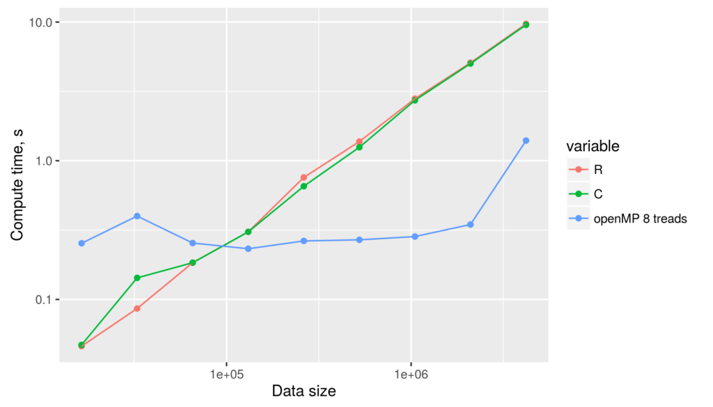
As an extended timing example, we run all the (optimized) examples above using a Xeon-L5420 cpu with 8 cores, single thread per core. The figure below depicts the compute time for single-threaded R and C++ code, and for C++/openMP code with 8 threads, as a function of data size.  The figure reveals several facts. First, for non-parallelized code we can see that
- Optimized R and C++ code are of virtually identical speed.
- compute time grows linearily in data size.
For openMP code the figure tells
- openMP with 8 threads is substantially slower for data size less than about 100k. For larger data, multi-threaded approach is clearly faster.
- openMP execution time is almost constant for data size up to 4M. For larger data vectors, it increases linearily. This suggests that for smaller data size, openMP execution time is dominated by thread creation and management overheads, not by computations.
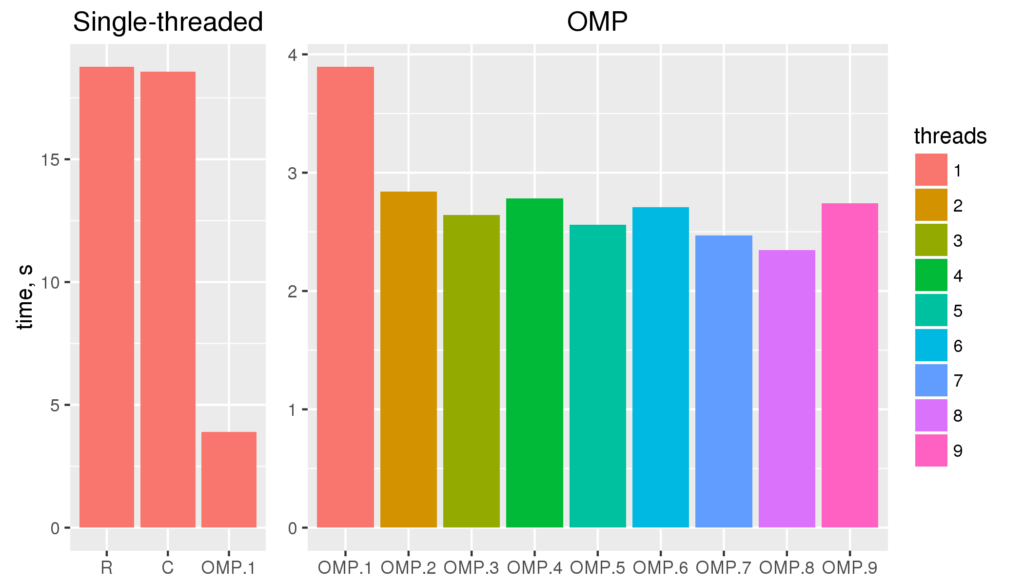
Finally, let’s compare the computation times for different number of threads for 8M data size.  The figure shows the run time for single threaded versions of the code (R and C), and multi-threaded openMP versions with 1 to 9 threads (OMP.1 to OMP.9).
- More cpus give us shorter execution times. 1-thread OMP will run almost 1.7 times slower than 8-threaded version (3.9 and 2.3 s respectively).
- The gain of more cpu cores working on the problem levels off quickly. Little noticeable gain is visible for more than 3 cores. It indicates that the calculations are only partly limited by computing-power. Another major bottleneck may be memory speed.
- Last, and most strikingly, even the single threaded OMP version of the code is 4.8 times faster than single-threaded C++ version with no OMP (18.6 and 3.9 s respectively)! This is a feature of the particular task, the compiler and the processor architecture. OMP parallel for–loops allow the compiler to deduce that the loops are in fact independent, and use faster SSE instruction set. This substantially boosts the speed but requires more memory bandwidth.
Conclusion
With the examples above I wanted to show that for many tasks, openMP is not hard to use. If you know some C++, parallelizing your code may be quite easy. True, the examples above are easy to parallelize at R-level as well, but there are many tasks where this is not true. Obviously, in the text above I just scratched the surface of openMP. If you consider using it, there are many excellent sources on the web. Take a look!
I am grateful to Peng Zhao for explaining the parallel loops and SSE instruction set.