This article is originally published in Capital of Statistic by Chinese [link] and I would like to thank He Tong for lots of great suggestions. All code in this post can be found on GitHub [link].

Data scientists are already very familiar with statistical software like R, SAS, SPSS, MATLAB; however, some of them are relatively inexperienced in parallel computing. So, in this post, I will introduce you some basic concepts on the use of parallel computing in R.

What is Parallel Computing？

Parallel computing, specifically, should include high-performance computers and parallel software. The peak performance of high-performance computers increases quickly. In the most recent ranking of the world’s TOP500 supercomputers, Chinese Sunway Taihu Light topped the list with 93 PFLOPS (here). For most individuals, small and medium enterprises, high-performance computers are too expensive. So, the application of high-performance computers is indeed limited, mainly in the field of national defense, military, aerospace and research areas. In recent years, with the rapid developments of multicore CPU, cheap cluster, and various accelerators (NVIDIA GPU, Intel Xeon Phi, FPGA), personal computers has been comparable to high-performance computers. 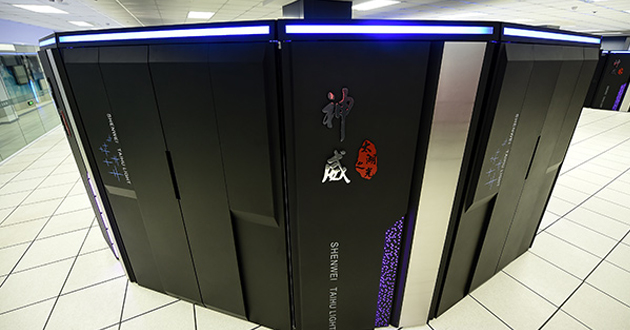On the other hand, the software changes lag a lot. Imagine what software you’re using supported parallel operations, Chrome, Visual Studio or R? Software parallelization requires more research and development supports. It is called code modernization for the procedure of changing the serial code to parallel, which sounds a very interesting work. But, in practice, a large number of bug fixes, data structure rewrite, uncertain software behaviors and cross-platform issues greatly increase the software development and maintenance costs.

Why R Needs Parallel Computing?

Let’s come back to R. As one of the most popular statistical software, R has a lot of advantages, such as a wealth of statistical models, data processing tools, and powerful visualization capabilities. However, with an increasing amount of data, R’s memory usage and computation mode limit R to scale. From the memory perspective, R uses in-memory calculation mode. All data need to be processed in the main memory (RAM). Obviously, its advantages are high computational efficiency and speed, but the drawback is that the size of the problem can be handled by R is very limited (<RAM ). Secondly, R core is a single-threaded program. Thus, in the modern multi-core processors, R can not effectively use all the computing cores. If the R went to the Sunway CPU of 260 computing cores, single-threaded R only take 1/260 computing power and waste other computing cores of 259/260.

Solution？Parallel Computing!

Parallel computing technology can solve the problem that single-core and memory capacity can not meet the application needs. Thus, the parallel computing technology will be extremely expansion of the use of R. From R 2.14 (Feb 2012), ‘parallel‘ package is installed by default. Obviously, R core development team also attached great importance to parallelization.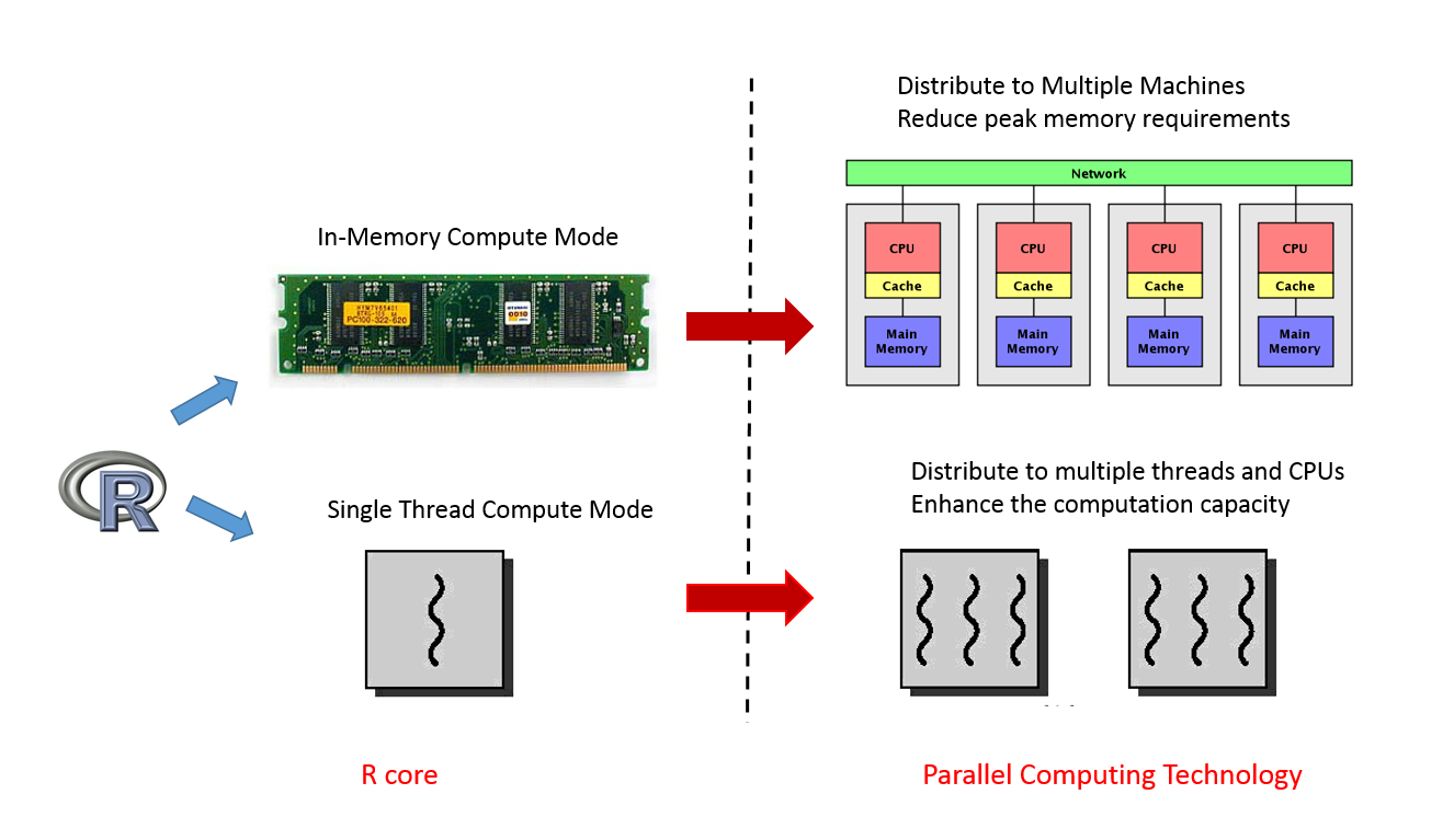

How to Use Parallel Computing?

From the user’s view, parallel computing in R can be divided into implicit and explicit computing mode.

Implicit Mode

Implicit computing hides most of the details for the user. It is not necessary to know how to allocate hardware resources, distribute workloads and gather results. The computations will start automatically based on the current hardware resources. Obviously, this mode is the most favorable. We can achieve higher performance without changing the calculation mode and our codes. Common implicit parallel mode includes:

Using Parallel Libraries

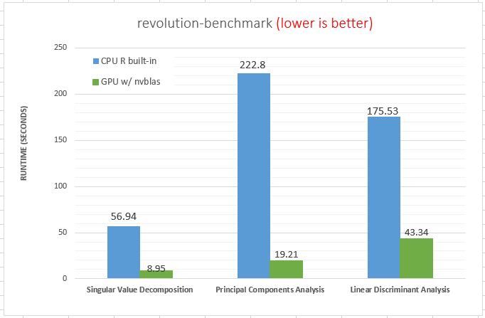
Parallel libraries, such as Intel MKL，NVIDIA cuBLAS, OpenBLAS are usually provided by the hardware manufacturer with in-depth optimizations based on the corresponding hardwares, so its performance is hugely better than R libraries. It is recommended choosing a high-performance R library at compile time or loading by LD_PRELOAD at runtime. The details of compiling, loading and using BLAS libraries can be found in the one of our previous blog (in here). In the first diagram, the matrix calculation experiments, parallel libraries on 1 or 2 CPUs is a hundred times faster than R original library. On the second, we can see the GPU math library shows remarkable speed for some common analysis algorithms as well. 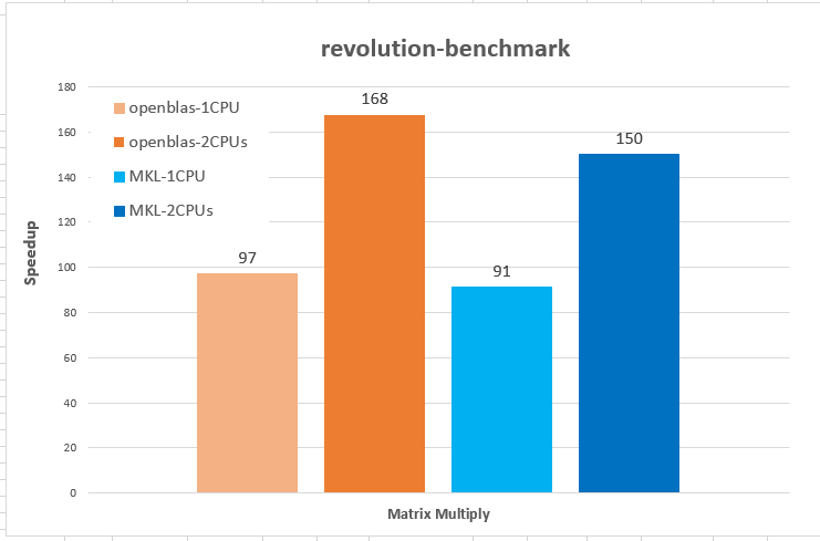Now, let’s run an interesting example in which we didn’t call GEMM function explicitly but still get lots of performance improvements from parallel BLAS library. In below example, we train MNIST dataset by DBN,deep belief network, (SRBM,Stacked Restricted Boltzmann Machine ) with deepnet package. This example refers the blog of “training MNIST data with the package deepnet“ where the author got the accuracy of 0.004% on training data and 2% on testing data. Because the original network of c(500,500,250,125) is too huge to run, I simplified the network architecture in our case and the code of deepnet_mnist.R in here.

#install.packages("data.table")
#install.packages("deepnet")
 
library(data.table)
library(deepnet)
 
# download MNIST dataset in below links
# https://h2o-public-test-data.s3.amazonaws.com/bigdata/laptop/mnist/train.csv.gz
# https://h2o-public-test-data.s3.amazonaws.com/bigdata/laptop/mnist/test.csv.gz
mnist.train <- as.matrix(fread("./train.csv", header=F))
mnist.test  <- as.matrix(fread("./test.csv", header=F))
 
# V785 is the label
x <- mnist.train[, 1:784]/255
y <- model.matrix(~as.factor(mnist.train[, 785])-1)
 
system.time(
    nn <- dbn.dnn.train(x,y,
                        hidden=c(64),
                        #hidden=c(500,500,250,125),
                        output="softmax",
                        batchsize=128, 
                        numepochs=100, 
                        learningrate = 0.1)
)

Thus, we run this piece of code twice. We got 3.7X **and **2.5Xspeedup (runtime of 2581 sec .vs. 693 sec and 1213 sec ) by Intel MKL and OpenBLAS library on Intel SandyBridge E-2670.

> R CMD BATCH deepnet_mnist.R
> cat deepnet_mnist.Rout
deep nn has been trained.
     user system   elapsed 
 2574.013  1.404  2581.882
 
> env LD_PRELOAD=/.../tools/OpenBLAS/lib/libopenblas.so R CMD BATCH deepnet_mnist.R
> cat deepnet_mnist.Rout
deep nn has been trained.
     user    system  elapsed 
 4752.005 25881.221 1213.644
 
# Compiled with Intel Compiler and MKL
> R CMD BATCH deepnet_mnist.R
> cat deepnet_mnist.Rout
deep nn has been trained.
      user  system elapsed 
 10770.641 290.486 693.146

Using MultiThreading Functions

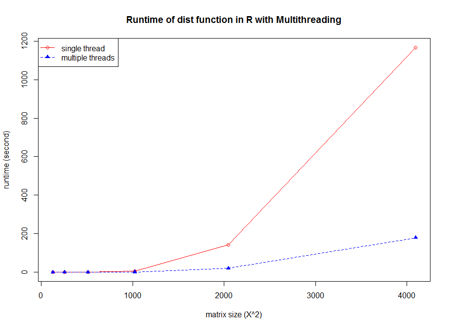
OpenMP is a multithreading library based on shared memory architecture for application acceleration. The latest R has been opened OpenMP options (-fopenmp) at compile time on Linux, which means that some of the calculations can be run in multithreaded mode. For example , dist is implemented by multithreading with OpenMP. The example code as below (ImplicitParallel_MT.R):

# Comparison of single thread and multiple threads run
# using Internal function to set thread numbers, not very grace, but don't find a good way till now.
# Ang suggestion?
setNumThreads <- function(nums=1) {
  .Internal(setMaxNumMathThreads(nums))
  .Internal(setNumMathThreads(nums))
}
 
# dataset from 2^6 to 2^11
for(i in 6:11) {
  ORDER <- 2^i
  m <- matrix(rnorm(ORDER*ORDER),ORDER,ORDER)
  setNumThreads(1)
  res <- system.time(d <- dist(m))
  print(res)
  setNumThreads(20)
  res <- system.time(d <- dist(m))
  print(res)
}

Using Parallel Packages

In the list of R high-performance computing, there are lots of parallel packages and tools. These parallel packages can be used like any other R packages quickly and conveniently. R users can always focus on the problem itself, without having to think too much about parallelism implementations and performance issues. Take H2O.ai for example, it takes Java as the backend to achieve multi-threading and multi-nodes computing. Users only need to load the package, and then initialize H2O with thread number. After that subsequent calculations, such as GBM, GLM, DeepLearning algorithm, will automatically be assigned to multiple threads and multiple CPUs.

library(h2o)
h2o.init(nthreads = 4)
# Connection successful!
# R is connected to the H2O cluster: 
# H2O cluster uptime: 1 hours 53 minutes 
# H2O cluster version: 3.8.3.3 
# H2O cluster name: H2O_started_from_R_patricz_ywj416 
# H2O cluster total nodes: 1 
# H2O cluster total memory: 1.55 GB 
# H2O cluster total cores: 4 
# H2O cluster allowed cores: 4 
# H2O cluster healthy: TRUE 
# H2O Connection ip: localhost 
# H2O Connection port: 54321 
# H2O Connection proxy: NA 
# R Version: R version 3.3.0 (2016-05-03)

Explicit Mode

Explicit parallel computing requires the user to be able to deal with more details, including data partitions, task distributions, and final results collections. Users not only need to understand their own algorithms but also need to have a certain understanding of hardware and software stack. Thus, it’s a little difficult for users. Fortunately, parallel computing framework in R, such as parallel,Rmpi and foreach, provides the simple parallel programming approach by mapping structure. R users only need to transfer the code into the form of *apply or for, and then replace them by parallel APIs such as mc*apply or foreach. For more complex calculation flow, the user can repeat the process of map-and-reduce. 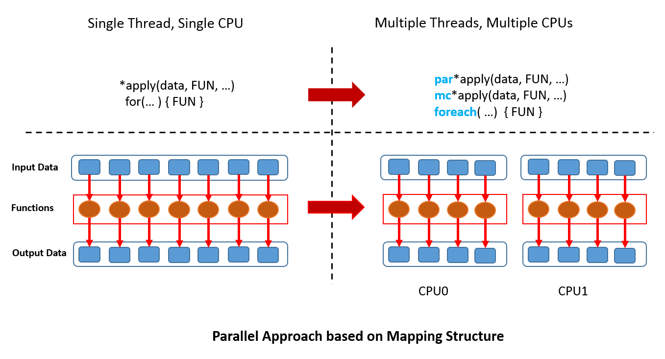Now, we show you a parallel example by solving quadratic equation with *apply and for style. The whole code in ExplicitParallel.R. First, we present a non- vectorized function for solving the equation, which can handle several special cases, such as second quadratic coefficient is zero, or second and first quadratic term are zero, or the number of the square root is negative.

# Not vectorized function
# Quadratic Equation: a*x^2 + b*x + c = 0
solve.quad.eq <- function(a, b, c) 
{
  # Not validate eqution: a and b are almost ZERO
  if(abs(a) < 1e-8 && abs(b) < 1e-8) return(c(NA, NA) )

  # Not quad equation
  if(abs(a) < 1e-8 && abs(b) > 1e-8) return(c(-c/b, NA))

  # No Solution
  if(b*b - 4*a*c < 0) return(c(NA,NA))

  # Return solutions
  x.delta <- sqrt(b*b - 4*a*c)
  x1 <- (-b + x.delta)/(2*a)
  x2 <- (-b - x.delta)/(2*a)

  return(c(x1, x2))
}

And then, we randomly generated three big vectors to storage three coefficients.

# Generate data 
len <- 1e8
a <- runif(len, -10, 10)
a[sample(len, 100,replace=TRUE)] <- 0
 
b <- runif(len, -10, 10)
c <- runif(len, -10, 10)

*apply IMPLEMENTATION:

First, we look at the serial code. The data is mapped into solver function,solve.quad.eq by lapply, and the results are saved into list finally.

# serial code
system.time(
  res1.s <- lapply(1:len, FUN = function(x) { solve.quad.eq(a[x], b[x], c[x])})
)

Next, we use the function of mcLapply (multicores) in parallel package to parallelize calculations in lapply. From the API interface, the usage of mcLapply is really similar with lapply in addition to specifying the core numbers. mcLapply creates multiple copies of the current R session based on Linux fork mechanism, and evenly assign compute tasks into multiple processes regarding with input index. Finally, the master R session will collect the results from all worker sessions. If we specify two worker processes, one process calculated 1:(len/2) while another computing (len/2+1):len, and finally two parts of results will be merged into res1.p. However, due to the use of Linux mechanisms, this version can’t be executed on Windows platform.

# parallel, Linux and MAC platform
library(parallel)
# multicores on Linux
system.time(
  res1.p <- mclapply(1:len, 
                      FUN = function(x) { solve.quad.eq(a[x], b[x], c[x]) }, 
                      mc.cores = 4)
)

For non-Linux users, we can use parLapply function in parallel package to achieve parallelism. parLapply function supports different platforms including Windows, Linux and Mac with better portability, but its usage is a little complicated than mclapply. Before using parLapply function, we need to create a computing group (cluster) first. Computing group is a software-level concept, which means how many R worker processes we need to create (Note: par*apply package will create several new R processes rather than copies of R master process from mc*apply). Theoretically, the size of the computing group is not affected by the hardware configuration.For example, we can create a group with 1000 R worker processes on any machine. In practice, we usually use the same size of computing group with hardware resources (such as physical cores) so that each worker process of R can be mapped to a physical core. In the following example, we start with detectCores function to determine the number of computing cores in the machine.It is noteworthy that detectCores() returns the number of Hyper-Threading rather than real physical cores.For example, there are two physical cores on my laptop, and each core can simulate two hyperthreading , so detectCores() return value is 4. However, for many compute-intensive tasks, the Hyper-Threading is not much helpful for improving performance, so we use the parameter of logical=FALSE to get the actual number of physical cores and then create the same number group.Since the worker processes in the group is new R sessions, the data and functions of the parent process is not visible. Therefore, we have to broadcast the data and functions to all worker processes by clusterExport function. Finally parLapply will distribute the tasks to all R worker processes evenly, and then gather results back.

# cluster on Windows
cores <- detectCores(logical = FALSE)
cl <- makeCluster(cores)
clusterExport(cl, c('solve.quad.eq', 'a', 'b', 'c'))
system.time(
  res1.p <- parLapply(cl, 1:len, function(x) { solve.quad.eq(a[x], b[x], c[x]) })
)
stopCluster(cl)

for IMPLEMENTATION:

The computation approach of for is very similar with *apply. In the following serial implementation, we created a matrix for storage results and update the results one by one in the inner loop.

# for style: serial code
res2.s <- matrix(0, nrow=len, ncol = 2)
system.time(
  for(i in 1:len) {
      res2.s[i,] <- solve.quad.eq(a[i], b[i], c[i])
  }
)

For the for loop parallelization, we can use %dopar% in foreach package to distribute the computations to multiple R workers. foreach package provides a method of data mapping, but does not include the establishment of computing group.Therefore, we need to create a computing group by doParallel or doMC package. Creating computing group is as same as before, except setting backend of computations by registerDoParallel. Now we consider the data decomposition. Actually, we want each R worker process to deal with continuous computing tasks. Suppose we have two R worker processes, the process 1 computes from 1:len/2, another process for (len/2+1):len. Therefore, in the following example code, we evenly distribute the vectors to computing group and each process calculates the size of chunk.size. Another important skill is using local matrix to save partial results in each process. Last, combine local results together by .combine='rbind' parameter.

# foreach, work on Linux/Windows/Mac
library(foreach)
library(doParallel)
 
# Real physical cores in my computer
cores <- detectCores(logical = FALSE)
cl <- makeCluster(cores)
registerDoParallel(cl, cores=cores)
 
# clusterSplit are very convience to split data but it takes lots of extra memory
# chunks <- clusterSplit(cl, 1:len)
 
# split data by ourselves
chunk.size <- len/cores
 
system.time(
  res2.p <- foreach(i=1:cores, .combine='rbind') %dopar%
  { 
    # local data for results
    res <- matrix(0, nrow=chunk.size, ncol=2)
    for(x in ((i-1)*chunk.size+1):(i*chunk.size)) {
        res[x - (i-1)*chunk.size,] <- solve.quad.eq(a[x], b[x], c[x])
    }
    # return local results
    res
  }
)
 
stopImplicitCluster()
stopCluster(cl)

Finally, we tested the code on Linux platform with 4 threads and can gain more than **3X speedup ** for every parallel implementation!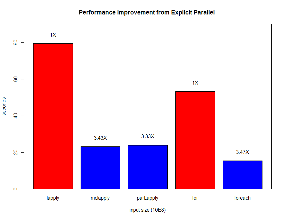

Challenges and Prospects

Challenges :In practice, the problem needed to be resolved by parallel computing is not such simple as our examples. To parallelize R and its eco-system are still very difficult because,

R is a decentralized and non-commercial software

R is not developed by a compact organization or company while most of R’s packages are contributed by users. It means that it is difficult to adjust and unify software architecture and design with the same philosophy. On the other hand, commercial software, such as Matlab, with unified development, maintenance, and management, can be relatively easier to restructure and reconstruct. Therefore, after several times update, the parallelism of commercial software will be much higher.

The infrastructure design of R is still single-threaded

R was originally designed for single-threaded so that many of the underlying data structures and functions are not thread-safe. Therefore, lots of codes need to be rewritten or adjust for high-level parallel algorithms. But it likely will destroy the original design patterns.

The packages are highly dependent

Assume that we use package B in R, and B depends on some functions of package A. If package B is improved by multithreading first; after that package A is also enhanced by parallelization. So, it is likely to appear hybrid parallel when we use package B. It may lead lots of strange errors (BUGs) and performance decrease if there is no comprehensive design and testing during developments. Prospects: How will the future of parallelism in R ?

High-performance components from commercial and research organizations

Essentially, software developments are inseparable from the human and financial investments. The packages, such as H2O, MXNet, Intel DAAL, improve the performance significantly from parallelism with long-term supports.

Cloud Platform

With the rise of cloud computing ,Data Analyst as a Services (DAAS) and Machine Learning as a Service (MLAS) are more and more popular.The major cloud providers optimize their tools, including R, from hardware deployments, database, high-level algorithms and explore much more parallelism in application level. For example, Microsoft recently launched a series supports for R in their cloud (here). Therefore, parallel in R will be more transparent. The user does the same things in R, but the real computing will be distributed to the cloud.

ParallelR

R with Parallel Computing from User Perspectives