R for Deep Learning (II): Achieve High-Performance DNN with Parallel Acceleration

I would like to thank Jun Ma and all other technical reviewers and readers for their informative comments and suggestions in this post.

50 years of Data Science, David Donoho, 2015

**Computing with Data.**Every data scientist should know and use several languages for data analysis and data processing. These can include popular languages like R and Python … Beyond basic knowledge of languages, data scientists need to keep current on new idioms for efficiently using those languages and need to understand the deeper issues associated with computational efficiency.

In the previous post, R for deep learning (I), I introduced the core components of neural networks and illustrated how to implement it from scratch by R. Now, I will focus on computational performance and efficiency of R’s implementation, especially for the parallel algorithm on multicores CPU and NVIDIA GPU architectures.

Performance Profiling

In this post, we are going to a little big dataset, MNIST, for performance analysis. MNIST widely used to measure the accuracy of classification by handwritten digits in machine learning field, and also used for the competition in Kaggle (data in download page or here). Yann has provided the classification results based on various machine learning algorithms on his page.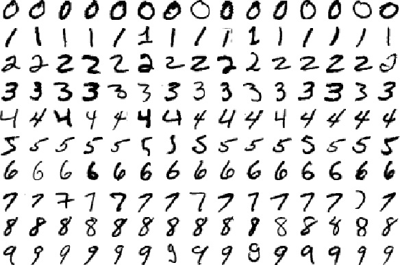

Picture.1 Handwritten Digits in MNIST dataset

The MNIST database contains 60,000 training images and 10,000 testing images. Each of image is represented by 28*28 points so totally 784 points. In this post, I will train the neural network with 784 points as input features and the number of 0-9 as output classes, then compare the runtime of our R DNN code with H2O deep learning implementations for 2-layers networks of the various number of hidden units (HU).

# h2o
library(h2o)
# single thread
h2o.init()
 
 
train_file <- "https://h2o-public-test-data.s3.amazonaws.com/bigdata/laptop/mnist/train.csv.gz"
test_file <- "https://h2o-public-test-data.s3.amazonaws.com/bigdata/laptop/mnist/test.csv.gz"
 
train <- h2o.importFile(train_file)
test  <- h2o.importFile(test_file)
 
# To see a brief summary of the data, run the following command
summary(train)
summary(test)
 
y <- "C785"
x <- setdiff(names(train), y)
 
# We encode the response column as categorical for multinomial
#classification
train[,y] <- as.factor(train[,y])
test[,y]  <- as.factor(test[,y])
 
# Train a Deep Learning model and valid
system.time(
  model_cv <- h2o.deeplearning(x = x,
                               y = y,
                               training_frame = train,
                               distribution = "multinomial",
                               activation = "Rectifier",
                               hidden = c(32),
                               l1 = 1e-5,
                               epochs = 200)
)

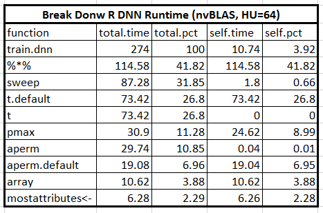
As I know, H2O is the fast and most popular deep learning package in R platform implemented by Java in the backend. Thus, it will be valuable to know how much performance gap between native R code and the mature package. As below barplot shown, the hidden units of 32, 64 and 128 are tested in 200 steps. 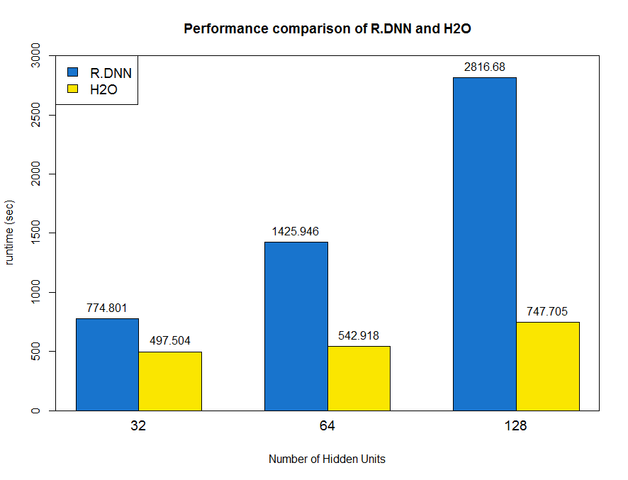Obviously, the R DNN is significantly slow than H2O, and the runtime increases with the number of hidden units quickly. For more details, we break down the R DNN runtime into each function call by Rprof() and summaryRprof() which report out the final results including 4 parts: total.time, total.pct, self.time and self.pct. The self.time and self.pct columns represent the elapsed time for each function, excluding the time from its inner called functions. The total.time and total.pct columns mean the total elapsed time for each function including the time spent on function calls [Aloysius Lim]. From the profiling results, we can see the top 1 time-consuming function is *“%%”** which represents matrix multiplications and usually people call it GEMM (GEneral Matrix Multiplication).

> Rprof()
> mnist.model <- train.dnn(x=1:784, y=785, traindata=train, hidden=64, maxit=200, display=50)
> Rprof(NULL)
> summaryRprof()
$by.self
                   self.time self.pct total.time total.pct
"%*%"                1250.08    90.19    1250.08     90.19
"t.default"            61.62     4.45      61.62      4.45
"pmax"                 24.40     1.76      28.42      2.05
"aperm.default"        11.60     0.84      11.60      0.84
"array"                10.36     0.75      10.36      0.75
"train.dnn"             9.74     0.70    1386.00    100.00
"<="                    5.72     0.41       5.72      0.41
"mostattributes<-"      4.02     0.29       4.02      0.29
"exp"                   3.60     0.26       3.60      0.26
"sweep"                 1.58     0.11     676.32     48.80
"is.data.frame"         1.28     0.09       1.28      0.09
"colSums"               0.86     0.06       0.86      0.06
"/"                     0.52     0.04       0.52      0.04
"rowSums"               0.36     0.03       0.36      0.03
"unname"                0.18     0.01       1.46      0.11
"-"                     0.04     0.00       0.04      0.00
"t"                     0.02     0.00      61.64      4.45
"sum"                   0.02     0.00       0.02      0.00
 
$by.total
                   total.time total.pct self.time self.pct
"train.dnn"           1386.00    100.00      9.74     0.70
"%*%"                 1250.08     90.19   1250.08    90.19
"sweep"                676.32     48.80      1.58     0.11
"t"                     61.64      4.45      0.02     0.00
"t.default"             61.62      4.45     61.62     4.45
"pmax"                  28.42      2.05     24.40     1.76
"aperm"                 21.96      1.58      0.00     0.00
"aperm.default"         11.60      0.84     11.60     0.84
"array"                 10.36      0.75     10.36     0.75
"<="                     5.72      0.41      5.72     0.41
"mostattributes<-"       4.02      0.29      4.02     0.29
"exp"                    3.60      0.26      3.60     0.26
"unname"                 1.46      0.11      0.18     0.01
"is.data.frame"          1.28      0.09      1.28     0.09
"data.matrix"            1.28      0.09      0.00     0.00
"colSums"                0.86      0.06      0.86     0.06
"/"                      0.52      0.04      0.52     0.04

Parallel Acceleration

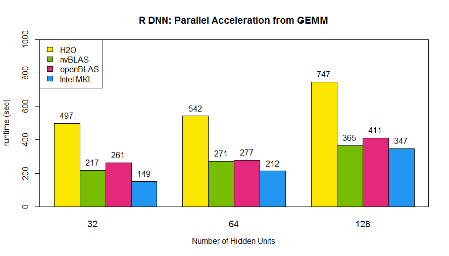
From above analysis, the matrix multiplication (“%*%”) accounts for about 90% computation time in the training stage of the neural network. Thus, the key of DNN acceleration is to speed up matrix multiplication. Fortunately, there are already several parallel libraries for matrix multiplication and we can deploy it to R easily. In this post, I will introduce three basic linear algebra subprograms (BLAS) libraries, openBLAS, Intel MKL, and cuBLAS. (In another blog, moreover, we show their performance on modern hardware architectures and instructions of installation). The former two are multithread accelerated libraries which need to be built with R together (instructions in here and here). On the other hand, it is indeed easy to apply NVIDIA cuBLAS library in R on Linux system by the drop-on wrap, nvBLAS, which can be preloaded into R in order to hijack original Rblas.so. By this way, we can leverage NVIDIA GPU’s power into R with zero programming efforts :) The below picture shows the architecture of R with BLAS libraries. Typically, R will call their own BLAS, Rblas.so,on Linux system which handles all kinds of linear algebra functions (here), but it is a single thread implementation. The trick to speed up the linear algebra calculations is to update the R standard BLAS to modern multithread libraries. For R developers, there is almost a ‘free lunch’ without rewriting their codes for parallel accelerations. 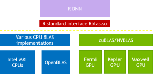As below code shown, we tested prebuilt R with openBLAS, Intel MKL and nvBLAS for 2-layers neural network of 32, 64 and 128 neurons.From the below bar chart, the runtime of R DNN are dramatically decreased and it is nearly 2X faster than H2O and 9X speedup (from 2816 to 365 for 128 hidden neurons network) than original R code!

# you must create a configuration file nvBLAS.conf in the current directory, example in here. >LD_PRELOAD=libnvblas.so /home/patricz/tools/R-3.2.0/bin/bin/R CMD BATCH MNIST_DNN.R

Note: Testing hardware: Ivy Bridge E5-2690 v2 @ 3.00GHz, dual socket 10-core (total 20 cores), 128G RAM; NVIDIA GPU K40m; Software: CUDA 7.5, OpenBLAS 0.2.8, Intel MKL 11.1

Optimization

Till now, it seems everything is great and we gain lots of performance increments from BLAS libraries under multicores CPU and NVIDIA GPU system. But can we do a little more for performance optimizations? Let’s look into the profiling again and probe the top performance limiters. The below table shows the breakdown of R DNN code under acceleration by nvBLAS where the GEMM performance is 10X faster ( from original 1250 to 114 seconds ). But the next two top time-consuming functions, “sweep()” and “t()”, account for 27% (self.pct) runtime.Therefore, it makes sense to do further optimization for them.

A question for readers: The total time of ‘sweep’ is 87.28 but the self-time is only 1.8, so what are the real computation parts and is it a reasonable choose to optimize it?

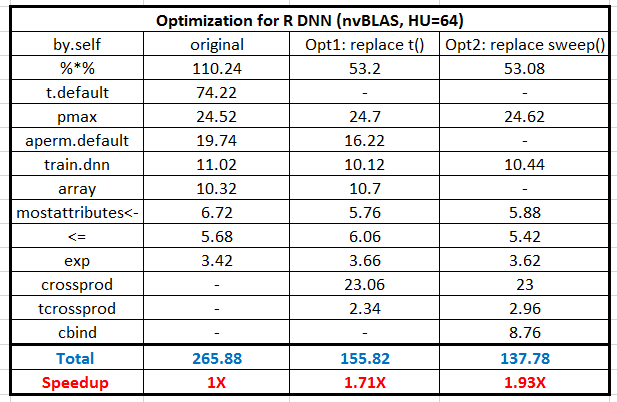
From the source code, there are several function calls of t() to transfer matrix before multiplication; however, R has already provided the inner function `crossprod` and `tcrossprod` for this kind of operations.

# original:  t() with matrix multiplication
dW2     <- t(hidden.layer) %*% dscores 
dhidden <- dscores %*% t(W2)

# Opt1: use builtin function
dW2     <- crossprod(hidden.layer, dscores)
dhidden <- tcrossprod(dscores, W2)

Secondly, the `sweep()` is performed to add the matrix with bias. Alternatively, we can combine weight and bias together and then use matrix multiplications, as below code shown. But the backside is that we have to create the new matrix for combinations of matrix and bias which increases memory pressure.

# Opt2: combine data and add 1 column for bias
#  extra matrix for combinations
X1   <- cbind(X, rep(1, nrow(X)))
W1b1 <- rbind(W1, b1)
W2b2 <- rbind(W2, b2)


# Opt2: remove `sweep` 
#hidden.layer <- sweep(X %*% W1 ,2, b1, '+')
hidden.layer <- X1 %*% W1b1

#score <- sweep(hidden.layer %*% W2, 2, b2, '+')
hidden.layer1 <- cbind(hidden.layer, rep(1,nrow(hidden.layer)))
score <- hidden.layer1 %*% W2b2

Now, we profile and compare the results again with below table. We save the computation time of ‘t.default’ and ‘aperm.default’ after removing ‘t()’ and ‘sweep()’ functions. Totally, the performance is DOUBLE again!

Another question: What is your opinion about the next step of optimizations? Any good idea and tell me your numbers :)

Summary

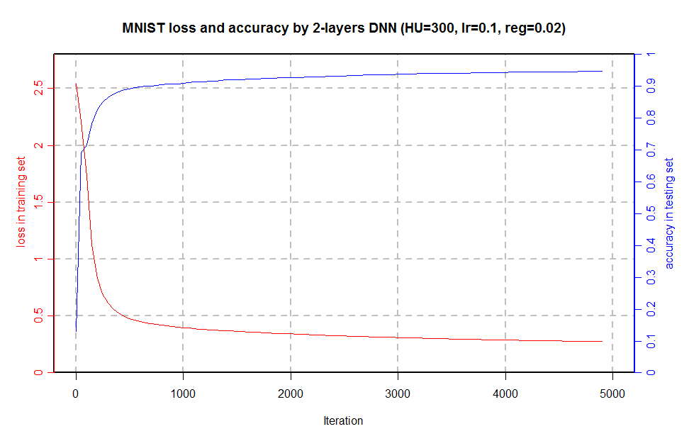
In this post, we have introduced the coarse granularity parallelism skill to accelerate R code by BLAS libraries on multicores CPU and NVIDIA GPU architectures. Till now, we have got +10X speedup under NVIDIA GPU and 2X faster than 20-threads H2O packages for a relatively small network; however, there are still lots of space to improve, take a try. 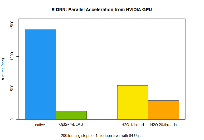And finally we train MNIST dataset with a 2 layer neural network of 300 hidden unit on Tesla K40m GPU, and we reach 94.7% accuracy (5.3% error rate) in an hour while Yann got 4.7% error rate with smaller learning rate ( lr=0.001) which will cost longer training time but more accurate. In the next blog post, I will continue deep learning topic and focus on CUDA integration and multiple GPUs accelerations.

Notes: 1. The entire source code of this post in here 2. The PDF version of this post in here 3. Pretty R syntax in this blog is Created by inside-R .org